BioHub Cell Tracking Working Note 1: Learned Lineage Graphs and Metric-Aware Repair

Series links and references
- Competition: BioHub - Cell Tracking During Development
- Official metric notes: RoyerLab kaggle-cell-tracking-competition metrics.md
- Background: Biohub Calls on AI Community to Transform 3D Cell Tracking
- Korean version: BioHub Cell Tracking 작업 기록 1: Lineage Graph 학습과 평가지표에 맞춘 후처리
- Follow-up: BioHub Cell Tracking Working Note 2: From a Leaderboard Plateau to OOF Structural Diagnostics
Related public notebooks
About this series. BioHub asks competitors to reconstruct cell lineage graphs from 3D microscopy movies. The labeled training set contains 199 movies from two embryos; Public scores cover 29% of the hidden test set, and Private scores cover the remaining 71%. The hidden test comes from embryos not seen in training. Each note follows the record through its stated period; later findings and retrospective comments are marked separately.
Later context — September 23, 2026. The July 18 metric patch tightened division matching after this note was written. Public differences within ±0.002 are read here as ties, under the project rule adopted on September 5–6; that was not the rule used to choose July submissions.
The first phase moved from classical centroid detection and nearest-neighbor links to a learned lineage graph with conservative repairs. By July 11, the useful unit of improvement was the submitted graph: a better detector or edge score mattered only if the graph builder and repair stages turned it into correct tracks.
A graph \(G=(V,E)\) represents each detected cell at one time as a node and each temporal link as an edge. A cell division appears as a fork. Under sparse annotation, a visually plausible cell may be unlabelled, and a missing intermediate detection can break an otherwise correct lineage. The metric therefore shapes both training and repair.
This note records the pipeline and early Public observations through July 11. Its final out-of-fold (OOF) section proposes a validation design in which each movie is predicted by a model trained without it; those evaluations had not yet been completed.
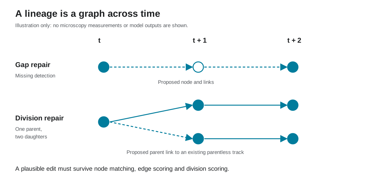 Figure 1. Schematic, not measured data. Gap repair inserts a missing node and its links. Division repair here adds a parent link to an existing parentless daughter track; it does not create a new daughter detection.
1. Competition Background
The competition asks participants to track fluorescently labeled cells in zebrafish embryo microscopy videos. Each sample is a short 3D time-lapse sequence. At every time point, the algorithm must detect cells in a 3D volume, link the same biological cell across time, and identify division events by reconstructing the lineage graph.
Cell positions alone do not explain development: the biological question is how cells move, divide, and form lineages over time. The hard part is that 3D microscopy data is dense, noisy, anisotropic, and visually repetitive. Many cells look alike. Cells may deform, disappear into dim regions, or divide into two daughters. Manual tracking becomes a bottleneck quickly.
The public data description gives the input contract:
1
2
3
4
5
6
7
8
9
10
11
sample.zarr/
  0/
    zarr.json
    c/{t}/0/0/0

shape: usually (T, Z, Y, X)
dtype: uint16
voxel scale:
  z = 1.62500 microns / voxel
  y = 0.40625 microns / voxel
  x = 0.40625 microns / voxel
Training samples also include sparse lineage annotations in GEFF format:
1
2
3
4
5
6
7
sample.geff/
  nodes/ids
  nodes/props/t/values
  nodes/props/z/values
  nodes/props/y/values
  nodes/props/x/values
  edges/ids
The important word is sparse. The annotations do not label every visible cell in every frame. That means ordinary dense segmentation validation can be misleading. A predicted cell can look reasonable in the image but still not correspond to a sparse ground-truth node. This pushes the workflow toward graph-level metrics and conservative post-processing.
The final submission is a single CSV with two row types:
1
2
3
4
id,dataset,row_type,node_id,t,z,y,x,source_id,target_id
0,44b6_xxxx,node,1,0,32,128,128,-1,-1
1,44b6_xxxx,node,2,1,33,130,125,-1,-1
2,44b6_xxxx,edge,-1,-1,-1,-1,-1,1,2
Node rows define cell detections. Edge rows define temporal links. The metric then interprets this CSV as a graph.
2. How the Metric Shapes the Graph
The official metric first matches predicted and ground-truth nodes per time point using physical centroid distance. The anisotropic voxel scale matters:
\[d_{\mu m}(i,j) = \sqrt{ (1.625\Delta z)^2 + (0.40625\Delta y)^2 + (0.40625\Delta x)^2 }.\]A node can match only if this physical distance is within the competition matching gate:
\[d_{\mu m}(i,j) \le 7.0.\]The scorer does not count every pair inside the radius as a match. At each frame \(t\), it finds an optimal bipartite assignment over admissible pairs, with each node matched at most once:
\[m_{ij}\in\{0,1\}, \qquad \sum_jm_{ij}\le1, \qquad \sum_im_{ij}\le1, \qquad m_{ij}=0\ \text{if}\ d_{\mu m}(i,j)>7.\]After node matching, a predicted edge is correct only when both endpoints match ground-truth nodes connected by a ground-truth edge. A ground-truth edge without such a prediction is a false negative. A predicted edge is a false positive only when its matched target belongs to another annotated source, or its matched source belongs to another annotated target. Other predicted edges, including edges outside the sparse annotated context, are ignored. For sample \(i\), the basic edge score is:
\[J_{\text{edge},i} = \frac{TP_i}{TP_i+FP_i+FN_i}.\]The node-count adjustment is also applied per sample. Let \(N_{\text{pred},i}\) be the predicted node count and \(N_{\text{total},i}\) the provided coarse estimate of all true cells, including unannotated cells:
\[r_i = \frac{N_{\text{pred},i}-N_{\text{total},i}} {N_{\text{total},i}}.\]With the official coefficient \(a=0.1\), the adjusted score for one sample is:
\[J_{\text{adj},i} = \max\left( 0, J_{\text{edge},i}(1-0.1r_i) \right).\]Over-prediction gives \(r_i>0\) and lowers the score. Under-prediction can make the multiplier exceed one, but deleting nodes is not a free gain: missing nodes usually remove valid links and increase \(FN_i\).
The aggregate edge score is not an unweighted mean over samples. It uses each sample’s Jaccard denominator,
\[D_i=TP_i+FP_i+FN_i,\]as its weight:
\[J_{\text{edge}}^{\text{adjusted}} = \frac{\sum_iD_iJ_{\text{adj},i}} {\sum_iD_i}.\]Division scoring is separate. The description below records the rules used in early July. A ground-truth division is a fork in the lineage graph. Because the visible split time is subjective, the official metric allows a tolerance of one frame on either side of the annotated split. The predicted graph must cover the pre-split stage and touch both daughter lineages. More precisely, one predicted weakly connected component must touch the pre-stage and both daughter lineages and contain a node with out-degree two. The fork itself does not have to be a predicted node directly matched to the ground-truth divider. Division events are micro-averaged across samples:
\[J_{\text{division}} = \frac{\sum_iTP_i^{\text{div}}} {\sum_i\left(TP_i^{\text{div}}+FP_i^{\text{div}}+FN_i^{\text{div}}\right)}.\]The final score is:
\[S = J_{\text{edge}}^{\text{adjusted}} +0.1J_{\text{division}}.\]This equation shaped almost every decision in my notebook. Three consequences matter:
| Metric pressure | Modeling consequence |
|---|---|
| Edge Jaccard dominates | Link quality is more important than merely detecting many bright spots. |
| Node overprediction is penalized | Isolated noisy nodes and short fragments can hurt. |
| Division has low but nonzero weight | Recovered true divisions must outweigh added false divisions and edges. |
This is why the notebook gradually moved away from “detect as much as possible” and toward:
1
2
3
4
detect enough nodes
link them well
repair graph errors only when geometry supports the edit
prune fragments that are unlikely to produce true edges
3. The Data Model In Code
The most important local convention is to keep graph operations in original voxel coordinates and convert only distances to microns.
Show snippet: physical coordinate contract
1
2
3
4
5
6
7
8
9
10
11
import numpy as np

VOXEL_SCALE_UM = np.array([1.625, 0.40625, 0.40625], dtype=np.float32)

def distance_um(a_zyx, b_zyx):
    a = np.asarray(a_zyx, dtype=np.float32)
    b = np.asarray(b_zyx, dtype=np.float32)
    return float(np.linalg.norm((a - b) * VOXEL_SCALE_UM))

def within_match_gate(a_zyx, b_zyx, gate_um=7.0):
    return distance_um(a_zyx, b_zyx) <= gate_um
This small contract prevents a surprisingly common error. The \(z\) axis is about four times coarser than \(x\) and \(y\). Treating voxel distance as Euclidean distance in raw index space can make the linking gate physically wrong.
4. First Baseline: Classical Centers And Nearest Links
The data contract, EDA, and classical baseline from this stage are available in Biohub Cell Tracking: Data Model, EDA, Baseline.
The first useful baseline was intentionally simple:
1
2
3
4
5
6
7
read one 3D frame
-> normalize intensity
-> find bright local maxima
-> refine centroids
-> remove duplicates by physical NMS
-> link adjacent frames by Hungarian matching
-> write nodes and edges
The baseline was not expected to win. It was useful because it made the metric visible. When node count exploded, the score fell. When links were too wide, false edges accumulated. When border peaks were left unchecked, many components became one-frame noise.
The key classical refinements were:
Intensity-weighted centroid refinement
For a coarse peak, refine its coordinate inside a local window \(W\):
\[\hat{\mathbf r} = \frac{ \sum_{\mathbf r\in W} \mathbf r \max(I(\mathbf r)-P_{20}(I_W),0) }{ \sum_{\mathbf r\in W} \max(I(\mathbf r)-P_{20}(I_W),0) }.\]Physical NMS
Two peaks that collapse to the same physical neighborhood should not both survive:
\[d_{\mu m}(i,j) < r_{\text{nms}}, \quad s_i\ge s_j \Longrightarrow \text{remove peak }j.\]Count stabilizer
A threshold failure in one frame can create a burst of false nodes. A simple guard is:
\[K_t=\min\!\left(N_t,\left\lceil\alpha N_{t-1}+\beta\right\rceil\right), \qquad\text{keep the }K_t\text{ strongest candidates in frame }t.\]
These steps control duplicate detections, unstable candidate counts, and coordinate errors before graph construction.
5. Learned Graph Model: UNet, Node Transformer, ILP
An integer linear program (ILP) selects a consistent graph from learned node and edge scores. I use anchor for the reference configuration against which a change is compared.
The stronger system uses the official learned-model family as the graph backbone. The conceptual pipeline is:
1
2
3
4
5
6
7
3D image volume
-> temporal UNet center detector
-> candidate cell nodes
-> node features and learned edge probabilities
-> ILP graph selection
-> output graph repair
-> submission.csv
The detector produces a center probability field:
\[p_t(\mathbf r) = \sigma \left( f_\theta(X_{t-k:t+k})(\mathbf r) \right),\]where \(X_{t-k:t+k}\) is a short temporal context around frame \(t\).
The learned edge model produces a logit for each candidate pair:
\[z_{ij} = g_\phi(h_i,h_j,\Delta t,\Delta \mathbf r).\]Here \(h_i\) and \(h_j\) are learned node representations. The logits are normalized and passed to an optimization layer rather than accepting every edge independently. That matters because a lineage graph has structural constraints. A node should not have arbitrary many parents. Division-like forks should be rare and physically plausible.
5.1 Combining Learned Edges With Motion Geometry
The post-link assignment does not use learned probability alone. When the previous displacement of source node \(i\) is available, its next position is predicted as:
\[\hat p_i = p_i+\lambda(p_i-p_{i-1}).\]The assignment cost for candidate target \(j\) is:
\[C_{ij} = \|p_j-\hat p_i\|_2 +0.05\|p_j-p_i\|_2 -\beta q_{ij}.\]Here \(q_{ij}\) is the learned edge probability and \(\beta\) determines how strongly learned evidence resolves a geometric tie. The current anchor uses \(\lambda=0.5\) and \(\beta=0.75\). Pairs outside the physical gate receive a large cost, and Hungarian assignment selects a one-to-one matching.
Show snippet: learned-edge weighted motion assignment
1
2
3
4
5
6
7
8
9
10
11
12
13
14
15
16
17
18
19
20
21
22
23
24
25
26
27
28
29
import numpy as np
from scipy.optimize import linear_sum_assignment

def assignment_cost(source_pos, target_pos, previous_pos, edge_prob):
    predicted = source_pos
    if previous_pos is not None:
        predicted = source_pos + 0.5 * (source_pos - previous_pos)

    raw_distance = np.linalg.norm(target_pos - source_pos)
    motion_distance = np.linalg.norm(target_pos - predicted)
    return motion_distance + 0.05 * raw_distance - 0.75 * edge_prob

cost = np.full((len(source_ids), len(target_ids)), LARGE_COST)
for i, source_id in enumerate(source_ids):
    for j, target_id in enumerate(target_ids):
        if raw_distance_um(source_id, target_id) <= gate_um:
            cost[i, j] = assignment_cost(
                position_um[source_id],
                position_um[target_id],
                predecessor_position_um.get(source_id),
                learned_edge_prob(source_id, target_id),
            )

rows, cols = linear_sum_assignment(cost)
matches = [
    (source_ids[i], target_ids[j])
    for i, j in zip(rows, cols)
    if cost[i, j] < LARGE_COST
]
This equation also explains the parameter sensitivity. If \(\beta\) is too small, the system becomes almost a nearest-motion tracker. If it is too large, an imperfectly calibrated learned score can override good geometry.
6. Why Graph Repair Became The Main Lever
An executable public version of the learned graph and gap-recovery family is available in Biohub Cell Tracking: Learned Graph w Gap Recovery.
Once the learned model became strong enough, broad detection changes became risky. The most useful changes moved to the graph level:
1
2
3
4
5
remove short noisy components
relink physically plausible motion breaks
recover one-frame gaps only when the midpoint is supported
add division edges only under strict geometry
avoid synthetic growth that inflates node count
The repair module I relied on most was short-track pruning. A connected component with only a few nodes often contributes no true edges but still increases the node count and edge false-positive surface.
The rule can be written as:
\[\operatorname{keep}(C) = \mathbf 1 \left[ |V_C|\ge L_{\min} \ \lor\ D_{\text{division}}(C)=1 \right].\]The snippet illustrates the rule with a default of 7. The \(0.900\) anchor in Section 9 used 6; the minimum length was set separately for each configuration.
Show snippet: short component pruning
1
2
3
4
5
6
7
8
9
10
11
def keep_component(component_nodes, component_edges, min_track_len=7):
    if len(component_nodes) >= min_track_len:
        return True

    # Do not remove a small component if it contains a plausible fork.
    out_degree = {}
    for source_id, target_id in component_edges:
        out_degree[source_id] = out_degree.get(source_id, 0) + 1

    has_fork = any(deg >= 2 for deg in out_degree.values())
    return has_fork
The experiment notes summarized pruning qualitatively:
| Minimum connected-component length | Recorded impression (no paired scores) |
|---|---|
| 4 | Useful, but leaves more short noise. |
| 6 | A useful setting in the recorded Public tests. |
| 7 | Competitive in other tests at the time. |
| 12 | Still viable, but begins to remove useful short tracks. |
| 14 | Over-pruning becomes visible. |
The exact number is not universal. It depends on the detector checkpoint, the hidden test distribution, and the rest of the repair stack. I retained moderate pruning as an empirical setting; its contribution still needed a paired local evaluation.
7. Gap Recovery And Safe Division
One-frame gap recovery tries to repair this pattern:
1
2
3
node at t
missing or weak node at t+1
node at t+2
The candidate midpoint is:
\[\mathbf m = \frac{\mathbf r_t+\mathbf r_{t+2}}{2}.\]The bridge is considered only if the displacement is physically plausible:
\[d_{\mu m}(\mathbf r_t,\mathbf r_{t+2}) \le 2r_{\text{gap}}.\]If an existing node is close to \(\mathbf m\), the notebook reuses it. Otherwise, it may create a synthetic midpoint and refine it from the image with a local intensity-weighted centroid. The synthetic shift is capped:
\[d_{\mu m}(\hat{\mathbf m},\mathbf m) \le r_{\text{shift}}.\]Synthetic growth is also capped globally:
\[N_{\text{synthetic}} \le \min \left( N_{\text{abs}}, \left\lfloor \rho |V| \right\rfloor \right).\]The important implementation detail is transactional rollback. If a repair is rejected, its inserted node must also be removed. Leaving an isolated node can worsen the node-count adjustment without recovering an edge.
Show snippet: one-frame gap insertion with rollback
1
2
3
4
5
6
7
8
9
10
11
12
13
14
15
16
17
18
19
20
21
22
23
24
25
26
27
28
29
30
31
32
33
34
35
36
37
38
39
def commit_gap_repair(
    source_id,
    target_id,
    source_point,
    target_point,
    t,
    endpoint_distance_um,
    nodes,
    edges,
    state,
):
    midpoint = 0.5 * (source_point + target_point)
    middle_id = find_reusable_isolated_node(midpoint, frame=t + 1)
    middle_reused = middle_id is not None

    if middle_id is None:
        if state.synthetic_added >= state.synthetic_cap:
            return False
        middle_id = next_node_id()
        refined = refine_with_local_intensity(midpoint, frame=t + 1)
        nodes[middle_id] = {
            "t": t + 1,
            "z": refined[0],
            "y": refined[1],
            "x": refined[2],
            "gap_synthetic": 1,
        }
        state.synthetic_added += 1

    needs_center = endpoint_distance_um >= 8.0
    if needs_center and center_score(nodes[middle_id]) < 0.20:
        if not middle_reused:
            nodes.pop(middle_id)
            state.synthetic_added -= 1
        return False

    edges.append((source_id, middle_id))
    edges.append((middle_id, target_id))
    return True
Division recovery is even more conservative. For a parent \(p_t\), an existing child \(c^{(1)}_{t+1}\), and a candidate second child \(c^{(2)}_{t+1}\), the edit is allowed only when:
\[d_{\mu m}(p,c^{(2)})\le r_{\text{parent}},\] \[d_{\mu m}(c^{(1)},c^{(2)})\le r_{\text{sister}},\]and the candidate child has no existing parent.
The reason is metric pressure. False-positive division edges can damage the division term and also create bad temporal edges. A division edit must recover enough true structure to offset any additional false edges and divisions. The break-even precision depends on the current graph and metric counts.
8. Objectives For Sparse Lineage Labels
Sparse labels make unlabelled bright cells uncertain negatives. Detection and association losses therefore limit negative supervision, while the ILP enforces a consistent graph. The equations below document those training objectives.
Training objectives and implementation details
The Temporal UNet and node Transformer are trained jointly for detection and association:
\[\mathcal L = \mathcal L_{\text{edge}} + \lambda_{\text{det}}\mathcal L_{\text{det}}.\]8.1 Detection Loss
Let \(y(\mathbf r)=1\) at an annotated center voxel and zero elsewhere. Because the annotation is sparse, \(y=0\) does not necessarily mean background. Positive and negative terms are normalized separately, and the negative mass is scaled by a small \(\eta\):
\[w_+=\frac{1}{N_+}, \qquad w_-=\frac{\eta}{N_-},\] \[\mathcal L_{\text{det}} = -\sum_{\mathbf r} \left[ w_+y(\mathbf r)\log \sigma(s_{\mathbf r}) + w_-(1-y(\mathbf r))\log(1-\sigma(s_{\mathbf r})) \right].\]Annotated centers remain strong positives without turning every unannotated bright cell into a hard negative.
8.2 Edge Loss
Let \(Y_{ij}\) be the ground-truth transition matrix between consecutive frames. Only rows or columns participating in an annotated transition enter the sparse supervision mask:
\[\mathcal M_{ij} = \mathbf 1 \left[ \sum_kY_{ik}>0 \quad\lor\quad \sum_kY_{kj}>0 \right].\]Edge logits are normalized over the source-node axis:
\[q_{ij} = \frac{\exp z_{ij}} {\sum_k\exp z_{kj}}.\]Each target therefore competes for one parent, while one source can still score highly for two targets. This suppresses merges without removing the representation of division. The implementation uses focal BCE with \(\gamma=2\):
\[p^*_{ij} = Y_{ij}q_{ij}+(1-Y_{ij})(1-q_{ij}),\] \[\mathcal L_{\text{edge}} = -\frac{1}{|\mathcal M|} \sum_{(i,j)\in\mathcal M} (1-p^*_{ij})^2 \left[ Y_{ij}\log q_{ij} + (1-Y_{ij})\log(1-q_{ij}) \right].\]Show snippet: sparse edge supervision
1
2
3
4
5
6
7
8
9
10
11
12
import torch
import torch.nn.functional as F

def sparse_edge_loss(logits, target):
    active_rows = target.sum(dim=1) > 0
    active_cols = target.sum(dim=0) > 0
    mask = active_rows[:, None] | active_cols[None, :]

    probs = torch.softmax(logits, dim=0)
    bce = F.binary_cross_entropy(probs, target, reduction="none")
    p_t = probs * target + (1.0 - probs) * (1.0 - target)
    return (((1.0 - p_t) ** 2) * bce)[mask].mean()
8.3 What The ILP Adds
The neural score \(q_{ij}\) is local evidence, not a valid lineage graph by itself. At inference, binary variables \(x_{ij}\) select edges while appearance, disappearance, and division variables carry structural costs. A simplified objective is:
\[\min_{x,a,d,b} -\lambda_e\sum_{ij}q_{ij}x_{ij} +\lambda_a\sum_j a_j +\lambda_d\sum_i d_i +\lambda_b\sum_i b_i.\]The essential degree constraints are:
\[\sum_i x_{ij}\le1, \qquad \sum_j x_{ij}\le1+b_i, \qquad b_i\in\{0,1\}.\]The first inequality prevents merges; the second allows one child normally and two when node \(i\) is selected as a division.
8.4 Positive-Unlabelled Loss For The Center Model
The auxiliary DeepCenterUNet3D predicts a single-frame center heatmap. Let \(h(\mathbf r)\) be the target heatmap and \(Q_{0.4}(I)\) the 40th intensity percentile. Its voxel weight is:
\[w(\mathbf r) = \begin{cases} 12, & h(\mathbf r)>0.05,\\ 1, & I(\mathbf r)<Q_{0.4}(I),\\ 0.05, & \text{otherwise}. \end{cases}\]Dark background is a normal negative, while bright unlabelled regions are nearly ignored:
\[\mathcal L_{\text{center}} = \frac{ \sum_{\mathbf r}w(\mathbf r) \operatorname{BCEWithLogits}(s_{\mathbf r},h(\mathbf r)) }{ \sum_{\mathbf r}w(\mathbf r) }.\]Show snippet: positive-unlabelled weighting
1
2
3
4
5
6
7
8
9
10
11
12
13
import numpy as np
import torch
import torch.nn.functional as F

weight_map = np.full(target_heatmap.shape, 0.05, dtype=np.float32)
background_cutoff = np.quantile(image, 0.40)
weight_map[image < background_cutoff] = 1.0
weight_map[target_heatmap > 0.05] = 12.0

target = torch.from_numpy(target_heatmap).to(logits)
weights = torch.from_numpy(weight_map).to(logits)
loss = F.binary_cross_entropy_with_logits(logits, target, reduction="none")
loss = (loss * weights).sum() / weights.sum().clamp(min=1.0)
The Center model does not replace the temporal graph. Its tested role was to supply image-space evidence for marginal repairs proposed by the temporal model.
9. Score Progression And What It Taught Me
The table compares complete submitted configurations through July 11. Some changed checkpoints and repairs together, so their score differences cannot identify each component’s contribution.
| Stage | Public LB reading | What changed |
|---|---|---|
| Classical and early lineage baselines | 0.68–0.75 | Validated the schema, physical distances, and graph output. |
| Strong rule-based geometry | 0.82–0.86 | Conservative topology went surprisingly far without a model artifact. |
| First learned artifact reproduction | about 0.81 | Reproducing a learned model was not enough by itself. |
| Learned graph plus graph repair | 0.844–0.860 | The combined repair configurations scored higher in these Public comparisons. |
| Checkpoint-specific graph calibration | 0.885–0.897 | Treated the checkpoint and post-processing as one system. |
| UNET400, spatial TTA, min-track 6 anchor | 0.900 | The tested broad recall expansions did not beat this configuration. |
| Conditional UNET400 + Center400 gap confirmation | 0.901 | Within 0.001 of the anchor; a tie under the later reading rule. |
9.1 Epoch Count Was Not An Independent Performance Axis
Comparing checkpoints around 125, 200, 250, 300, and 400 epochs produced an important result: more epochs did not automatically improve the Public score under fixed post-processing. A later checkpoint can have a lower internal loss while shifting detection and edge-probability calibration. I therefore treat a checkpoint as:
1
2
3
4
5
6
model weights
+ detector threshold
+ TTA contract
+ motion/edge assignment
+ repair caps
+ pruning length
not as weights alone. For example, moving the detector threshold from the \(0.9700\) anchor to \(0.9675\) and \(0.9725\) produced \(0.899\) on both sides. I stopped that narrow threshold sweep. The two readings are ties with the anchor under the later rule, leaving the threshold ordering unresolved.
9.2 Error Anatomy: 300ep Versus 400ep
Running the 300- and 400-epoch models over the same 199 training movies gave:
| Run | Edge TP | Edge FP | Edge FN | Global edge J | Mean score proxy |
|---|---|---|---|---|---|
| UNET300 | 121,669 | 5,212 | 7,214 | 0.907334 | 0.902110 |
| UNET400 | 122,151 | 5,202 | 6,732 | 0.910997 | 0.912574 |
UNET400 gained 482 true-positive edges, removed 482 false negatives, and reduced false positives by 10. At the sample level, 101 movies improved and 86 worsened. The 400-epoch model was therefore not merely a more confident copy of the same predictor. Its aggregate in-sample counts improved and its error distribution changed. This made calibration mismatch a plausible reason for a threshold to transfer poorly, without isolating that cause.
There is an important qualification. Both checkpoints were trained on all training movies, so this was in-sample error anatomy, not true OOF evaluation. That distinction became essential when designing a learned repair policy.
10. What Did Not Work Yet
The failed experiments clarified how much authority each signal should receive.
10.1 Broad Recall And Aggressive TTA
Intensity TTA and aggressive detection expansion increased node counts without beating the best graph. One intensity-TTA branch fell to \(0.894\). Six-view spatial TTA using flips and XY rotations was useful, but more views were not automatically better.
10.2 An edge_predictor Checkpoint Is Not Just An Edge Head
One of the largest failures came from swapping a separate edge_predictor_best.pth into the calibrated graph. The filename suggests an edge scorer, but the checkpoint contains the full model state, including the TemporalUNet detector.
| Output | Calibrated UNET400 anchor | Uncalibrated checkpoint swap |
|---|---|---|
| Node rows | 128,535 | 170,860 |
| Edge rows | 123,988 | 164,603 |
| Public score | about 0.900 | 0.861 |
Nodes and edges increased by roughly 33%. The new checkpoint had inherited the old \(0.97\) detection threshold and configuration without recalibration. This showed that an independent-seed model should not be submitted as a blind weight swap. A changed checkpoint needs its own complete-pipeline evaluation. Section 12 proposes one way to compare and combine independently trained models.
10.3 Small ILP Changes Still Need Isolated Experiments
Lowering the division weight from \(1.0\) to \(0.7\) scored \(0.897\). The same notebook also contained a pool_kernel_um=2.0 patch, but it ran after prediction and therefore had no effect on the submission. Bundling changes into one cell can make execution order obscure what was actually tested.
10.4 Center Did Not Help As a Global Detector
DeepCenterUNet3D did not help as a blind union or as a hard gate over every synthetic node. Requiring Center confidence for all synthetic gap nodes scored \(0.898\), compared with \(0.900\) for the anchor and \(0.901\) for conditional confirmation. A genuinely missing cell is often dim or occluded, so the auxiliary detector can make the same false negative in the same difficult frame.
There was also an artifact trap. The best.pt files in the 100–500 epoch snapshots all referred to the same early best checkpoint. Testing a specific Center epoch required checkpoint_last.pt plus an explicit assertion on the stored epoch.
11. A Narrower Role for the Auxiliary Center Model
Conditional confirmation gave Center veto authority only over geometrically marginal one-frame gaps already proposed by the UNET400 graph. It extends the public Biohub Cell Tracking: Blend Preprocessings notebook.
For a track ending at \(t\) and another beginning at \(t+2\), the gap proposal is:
\[\tilde p_{t+1}=\frac{p_t+p_{t+2}}{2}.\]The tested UNET400 + Center400 policy was:
\[\operatorname{accept}(d,c)= \begin{cases} 1, & d<8\ \mu\mathrm{m},\\ \mathbf{1}[c(\tilde p_{t+1})\ge0.20], & 8\le d\le12\ \mu\mathrm{m},\\ 0, & d>12\ \mu\mathrm{m}. \end{cases}\]Here \(d=\|p_{t+2}-p_t\|_2\), and \(c\) is the DeepCenter probability near the proposed midpoint. This configuration scored \(0.901\). In contrast, requiring \(c\ge0.15\) for every synthetic gap node scored \(0.898\).
Conditional confirmation scored \(0.003\) above the all-gap veto; against the anchor, it was a tie under the later reading rule. This motivated a working hypothesis:
1
2
strong temporal geometry > weak negative Center evidence
marginal temporal geometry + positive Center evidence > geometry alone
A dim cell can receive a low Center score even when it is real. A high score may add useful image evidence when motion geometry is uncertain. That was the rationale for restricting the model’s authority.
Show snippet: conditional Center confirmation
1
2
3
4
5
6
def accept_gap(span_um, center_prob):
    if span_um < 8.0:
        return True
    if span_um > 12.0:
        return False
    return center_prob >= 0.20
I proposed three extensions, none yet tested: a distance-adaptive threshold, agreement between forward and backward motion predictions, and separate treatment of synthetic nodes versus observed isolated nodes. The first would use:
\[\tau_c(d) = 0.12 + \operatorname{clip} \left( \frac{d-8}{4}, 0, 1 \right) \cdot (0.28-0.12).\]With bidirectional temporal context, the forward and backward midpoint predictions can also be compared:
\[\hat p_f=2p_t-p_{t-1}, \qquad \hat p_b=2p_{t+2}-p_{t+3},\] \[e_{\text{cons}} = \|\hat p_f-\hat p_b\|_2.\]In this proposed rule, \(e_{\text{cons}}\le2.5\,\mu\mathrm{m}\) would let temporal agreement bypass the image-space veto.
Show snippet: adaptive Center gate and bidirectional consensus
1
2
3
4
5
6
7
8
9
10
11
12
13
14
15
16
17
18
19
20
21
22
23
24
25
26
27
28
import numpy as np

def adaptive_center_threshold(span_um):
    fraction = np.clip((span_um - 8.0) / 4.0, 0.0, 1.0)
    return 0.12 + fraction * (0.28 - 0.12)

def linear_context(previous_id, source_id, target_id, following_id):
    return (
        previous_id is not None
        and following_id is not None
        and out_degree[previous_id] == 1
        and in_degree[following_id] == 1
        and nodes[previous_id]["t"] + 1 == nodes[source_id]["t"]
        and nodes[target_id]["t"] + 1 == nodes[following_id]["t"]
    )

if linear_context(previous_id, source_id, target_id, following_id):
    forward_mid = 2.0 * position_um[source_id] - position_um[previous_id]
    backward_mid = 2.0 * position_um[target_id] - position_um[following_id]
    consensus_error = np.linalg.norm(forward_mid - backward_mid)
else:
    consensus_error = np.inf

if consensus_error <= 2.5:
    accept = True
else:
    threshold = adaptive_center_threshold(endpoint_distance_um)
    accept = center_probability >= threshold
These proposals restrict auxiliary-model authority according to the type of uncertainty.
12. Proposed Next Step: Model Diversity and Strict OOF
A second model can serve two different purposes. An independent seed trained on all data is useful for test-time disagreement and ensembling. Its predictions on training movies are not OOF. A learned repair policy requires separate fold-held-out models.
1
2
3
4
5
all-train independent seed
-> test-time consensus and disagreement features

two-fold held-out models
-> true OOF graph edits and repair-policy labels
Show snippet: true two-fold OOF capture contract
1
2
3
4
5
6
7
8
9
10
11
12
13
14
15
16
17
18
19
20
21
22
23
24
25
26
27
28
29
from collections import Counter

oof_predictions = []
holdout_coverage = Counter()

for fold in (0, 1):
    train_movies = split_manifest[fold]["train"]
    holdout_movies = split_manifest[fold]["test"]

    assert set(train_movies).isdisjoint(holdout_movies)
    # embryo_of is provided by the dataset manifest, not inferred from row order.
    assert {embryo_of[m] for m in train_movies}.isdisjoint(
        {embryo_of[m] for m in holdout_movies}
    )

    # The epoch is fixed before inspecting this outer holdout.
    fixed_epoch = 100
    weight = weights_root / f"split_{fold}" / "checkpoint_last.pth"
    assert checkpoint_metadata(weight)["epoch"] == fixed_epoch
    predictions = predict_graphs(
        movies=holdout_movies,
        weight_path=weight,
    )
    oof_predictions.extend(predictions)
    holdout_coverage.update(holdout_movies)

expected_movies = set(all_training_movies)
assert set(holdout_coverage) == expected_movies
assert all(count == 1 for count in holdout_coverage.values())
Using edge_predictor_best.pth selected on the outer holdout to predict that same holdout would leak epoch selection into OOF. Use a fixed-epoch last checkpoint, or select the epoch on a separate inner validation split inside each outer-training fold.
A probability blend can be written as:
\[p_{\mathrm{blend}} = \alpha p_{\mathrm{anchor}} + (1-\alpha)p_{\mathrm{seed}}, \qquad \alpha\in[0,1].\]A blend changes the distributions seen by ILP, pruning, gap recovery and division repair. The proposed test therefore needs to calibrate \(\alpha\) and the complete downstream parameter vector jointly on separated OOF data.
A true OOF repair table naturally contains:
| Proposal type | Label source |
|---|---|
| existing edge | whether matched GT nodes have the same edge |
| one-frame gap bridge | whether GT contains the length-2 path |
| division edge | whether GT contains the same fork |
| short-component keep/drop | whether the component produces matched true edges |
The feature vector for a candidate edge or repair action can stay close to the metric rather than containing raw pixels:
\[x_{ij} = \left[ q_{ij}, d_{\text{raw}}, d_{\text{motion}}, \operatorname{rank}_{ij}, \deg^+(i), \deg^-(j), \rho_i, \rho_j, t_{\text{norm}}, c_{ij} \right].\]Here \(c_{ij}\) is optional Center evidence and \(\rho\) is local density. A compact policy can then export:
\[P(y_{ij}=1\mid x_{ij}) = \sigma(w^\top x_{ij}+b).\]Show snippet: exported repair-policy contract
1
2
3
4
5
6
7
8
9
10
11
12
13
14
15
16
17
18
19
20
21
FEATURE_COLUMNS = [
    "edge_prob",
    "edge_dist_um",
    "motion_dist_um",
    "candidate_rank_dist",
    "source_out_degree",
    "target_in_degree",
    "source_density_7um",
    "target_density_7um",
    "t_norm",
    "center_support",
]

policy = {
    "feature_columns": FEATURE_COLUMNS,
    "mean": feature_mean.tolist(),
    "scale": feature_scale.tolist(),
    "coef": classifier.coef_[0].tolist(),
    "intercept": float(classifier.intercept_[0]),
    "threshold": float(oof_optimal_threshold),
}
The final question is:
1
2
Which proposed graph edits are metric-positive,
given geometry, model disagreement, and local image evidence?
The current direction is therefore:
1
2
3
4
keep the calibrated UNET400 graph as the anchor
use Center only for marginal repair confirmation
train an independent seed for output-level disagreement
build true OOF repair actions with two-fold models
Closing
The submitted lineage graph is the unit that the metric scores. Node detection, edge selection and repair therefore need to be evaluated together, with the coordinate conventions and matching rules fixed.
The next question was: which structural error can be corrected, by what evidence, and at what cost on an unseen embryo?
Working Note 2 develops the validation plan for that question.
Series:
- 1: Learned Lineage Graphs and Metric-Aware Repair
- 8: What Went Into Choosing the Final Two