ROGII Working Note (2편): Target-Free TVT Geosteering의 오차 해부

Posted Jul 3, 2026 Updated Jul 4, 2026

By Pilkwang Kim

30 min read

Series 1 읽기:

English version:
ROGII Working Note (Part 2): Error Anatomy of Target-Free TVT Geosteering

Kaggle 대회:
ROGII Wellbore Geology Prediction

Kaggle Working Note:
Working Note: Target-Free TVT Geosteering

핵심 참고 노트:
Georgy Mamarin — Stop reforking: the best GR fit is the wrong depth

Georgy Mamarin의 노트북은 이 글을 쓰는 데 중요한 전환점이었다. 특히 “GR matching cost가 낮다”는 사실이 곧 “올바른 지층 깊이를 찾았다”는 뜻은 아니라는 점을 명확히 해 주었고, 논의를 단순한 점수 refork에서 오차 구조의 분해로 옮기는 데 큰 도움이 되었다.

대회 배경: 이것은 깊이 예측이 아니라 지층 좌표 복원이다

Kaggle의 ROGII 대회 설명은 목표를 간단히 말한다. 각 horizontal well의 evaluation zone에 대해 TVT를 예측해야 한다. 하지만 이 한 문장만으로는 문제의 성격이 잘 드러나지 않는다. 여기서 TVT는 단순한 지표면 기준 절대 깊이가 아니라, well이 지층 column 안에서 어느 stratigraphic position을 지나고 있는지 나타내는 좌표에 가깝다.

실제 geosteering workflow에서도 lateral gamma log를 하나 이상의 typewell과 맞추고, 필요하면 segmenting, stretching/squeezing, faulting을 고려한다. 즉 이 문제를 도메인 관점에서 표현하면 “row마다 TVT를 회귀한다”보다 “horizontal trajectory를 typewell coordinate system 안에 배치한다”에 더 가깝다.

수식으로 쓰면 row-wise regression은 다음처럼 보인다.

\[\hat T_{w,i}=f(MD_{w,i},X_{w,i},Y_{w,i},Z_{w,i},GR_{w,i}).\]

하지만 geosteering 관점에서는 먼저 well 단위의 coordinate transform을 생각하는 편이 자연스럽다.

\[s_i=\frac{MD_i-MD_{start}}{MD_{end}-MD_{start}},\qquad \hat T_w(s_i)=\hat D_w+\hat\phi_w(s_i).\]

여기서 $\hat D_w$는 지층 column 안에서 well 전체가 어디에 착지했는지를 나타내는 datum이고, $\hat\phi_w$는 tail이 그 datum에서 어떻게 drift하는지를 나타낸다. 이 구조를 받아들이면, 좋은 모델은 단순히 row feature를 많이 넣는 모델이 아니라 datum, mode, shape를 서로 다른 증거로 다루는 모델이 된다.

이 글의 나머지 논의는 이 배경 위에서 출발한다.

0. Series 1 이후 달라진 점

첫 번째 글의 핵심은 ROGII를 평범한 표 형식 회귀 문제가 아니라, 정답 TVT를 보지 않고 지층 좌표를 맞추는 target-free stratigraphic alignment 문제로 봐야 한다는 것이었다. 당시의 관심은 다음 흐름에 가까웠다.

visible trajectory + GR + typewell + prefix TVT_input
-> target-free pseudo-path
-> residual correction
-> leakage-controlled submission

그 관점은 여전히 유효하다. 다만 이후 공개 노트북, 토론, refork 실험, 그리고 후속 노트를 거치면서 더 중요한 질문이 생겼다.

If the target-free framing is correct,
where does the remaining error actually live?

처음에는 이 질문을 단순히 “더 좋은 GR fit을 찾으면 되는가?”로 생각하기 쉽다. 하지만 Georgy Mamarin의 노트북은 아주 중요한 정정을 제시했다. 가장 좋은 GR fit이 항상 올바른 TVT depth를 뜻하지는 않는다. gamma-ray curve는 암상 변화의 바코드처럼 작동하지만, 반복되는 지층 motif 때문에 여러 depth에서 그럴듯하게 맞을 수 있다. 그러면 문제는 GR cost의 최솟값 하나를 고르는 것이 아니라, datum, mode ambiguity, shape error를 분리해서 읽는 문제가 된다.

이번 노트는 Series 1의 EDA를 다시 가져오되, 거기에 다음 세 가지 관점을 추가한다.

축	질문	결론
datum	수평정 tail 전체가 어느 TVT level에서 시작하는가?	prefix/heel calibration으로 많은 well에서 회수 가능하지만, 놓치면 MSE를 크게 지배한다.
mode	두 개 이상의 stratigraphic bundle 중 어느 쪽인가?	GR cost margin만으로는 단정하기 어렵다. posterior mean 형태의 hedge가 더 자연스럽다.
shape	datum을 맞춘 뒤 tail slope와 curvature는 어떻게 이어지는가?	실제로 남아 있는 중요한 과제이지만, MSE 기준으로는 residual datum miss보다 작다.

이 글은 최종 제출 레시피를 다시 쓰려는 글이 아니다. 오히려 반대에 가깝다. 점수 refork를 멈추고, 어떤 종류의 오차를 회수할 수 있으며 어떤 오차는 완충해야 하는지를 정리하려는 노트다.

1. 왜 tabular regression이 아닌가

ROGII의 target은 한 컬럼 TVT다. 그래서 처음 보면 MD, X, Y, Z, GR 같은 행별 feature를 넣고 row-wise regressor를 학습하면 될 것처럼 보인다.

하지만 각 row는 독립 표본이 아니다. 하나의 horizontal well을 따라 지나가는 궤적상의 한 지점이다. 따라서 예측 대상도 행별 숫자 하나라기보다 hidden tail 전체의 TVT path에 가깝다.

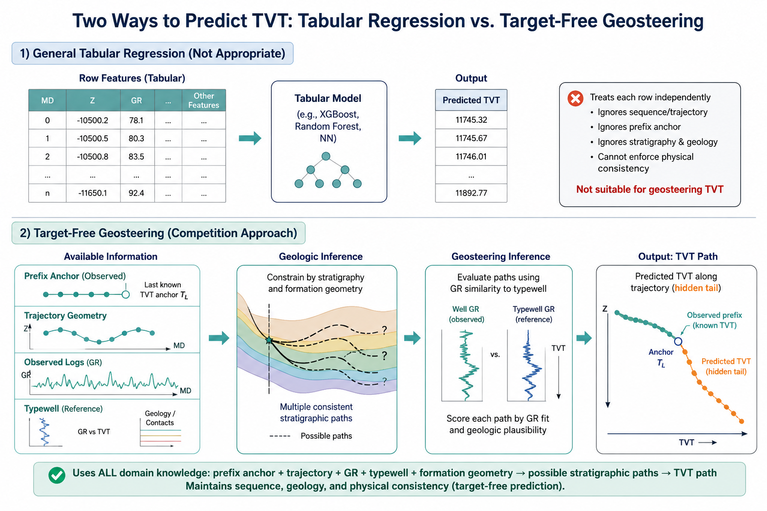
일반적인 row model은 다음 질문을 푼다.

\[\hat T_{w,i}=f(x_{w,i}).\]

반면 target-free geosteering은 well 단위의 hidden-tail 함수를 추정한다.

\[\hat T_w(s)=\hat D_w+\hat\phi_w(s),\qquad s\in[0,1].\]

여기서 $\hat D_w$는 well별 datum, $\hat\phi_w(s)$는 tail shape다. 핵심은 $\hat D_w$와 $\hat\phi_w$를 뒷받침하는 근거가 서로 다르다는 점이다.

구성	주로 읽는 근거
datum	prefix `TVT_input`, heel calibration, contact/formation prior
mode	GR/typewell likelihood landscape, PF/beam path, competing minima
shape	trajectory, `Z`, formation surface, low-order projection, residual model

이렇게 보면 모델은 하나의 black-box regressor가 아니라 여러 근거를 조합하는 경로 추정 시스템이다. row-wise model을 쓸 수는 있지만, 그것은 전체 path system의 일부로 들어가야 한다.

2. 정보 경계: 보이는 것과 숨겨진 것

Series 1에서 가장 중요했던 부분은 leakage boundary였다. 이번 글에서도 이 정보 경계가 모든 논의의 출발점이다.

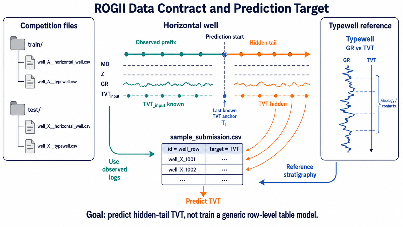
각 well $w$는 관측 가능한 prefix와 숨겨진 tail로 나뉜다.

\[\mathcal P_w=\{i:T^{input}_{w,i}\ \text{is observed}\},\qquad \mathcal H_w=\{i:T^{input}_{w,i}\ \text{is missing}\}.\]

제출해야 하는 행은 $\mathcal H_w$에 해당한다. 추정기가 사용할 수 있는 정보는 다음처럼 쓸 수 있다.

\[\hat T_{w,\mathcal H} =F\left( X_{w,\mathcal P\cup\mathcal H}, T^{input}_{w,\mathcal P}, \text{typewell}_w \right).\]

여기서 $X$는 MD/X/Y/Z/GR 같은 관측 공변량 trace다. 중요한 점은 full tail의 공변량은 Kaggle input으로 주어져 있으므로 batch setting에서는 사용할 수 있다는 것이다. 금지되는 것은 hidden target $T_{w,\mathcal H}$ 자체, 또는 그 target에서 파생된 통계량이다.

이 구분은 실제로 매우 중요하다.

신호	사용할 수 있는가?	이유
full horizontal GR trace	가능	test file에 주어진 공변량
typewell GR-vs-TVT curve	가능	기준 reference
prefix `TVT_input`	가능	visible anchor
hidden-tail `TVT`	불가	target
hidden-tail target mean / fitted oracle shape	불가	target에서 파생된 통계량
train-side oracle ladder	분석용 가능	inference feature가 아니라 ceiling 측정용

따라서 이 문제의 좋은 표현은 “future GR을 쓰면 leakage다”가 아니다. 더 정확한 표현은 다음이다.

Use future observed covariates if they are in the test file.
Do not use future target values, or summaries fitted from them.

실제 노트북에서는 이 경계를 먼저 코드 수준으로 고정했다. 핵심은 T_input이 보이는 prefix와 숨겨진 tail을 분리하고, tail target은 평가에만 쓰는 것이다.

  
is_prefix = horizontal["TVT_input"].notna()
prefix = horizontal.loc[is_prefix].copy()
tail = horizontal.loc[~is_prefix].copy()

safe_covariates = ["MD", "X", "Y", "Z", "GR"]
X_full = horizontal[safe_covariates]          # allowed: observed trace
T_prefix = prefix["TVT_input"]               # allowed: visible anchor
T_tail_true = tail["TVT"]                    # analysis / validation only

이 작은 분리가 중요하다. 많은 leakage는 복잡한 모델에서 생기는 것이 아니라, 이 경계를 흐리게 만드는 편의성 feature에서 시작한다.

3. Well-level EDA: anchor는 강하지만 완전하지 않다

학습 데이터의 hidden tail은 길다. 그래서 작은 datum error도 row-wise RMSE에서는 크게 누적된다. 이번 노트에서 다시 계산한 well-level summary는 이 점을 분명히 보여준다.

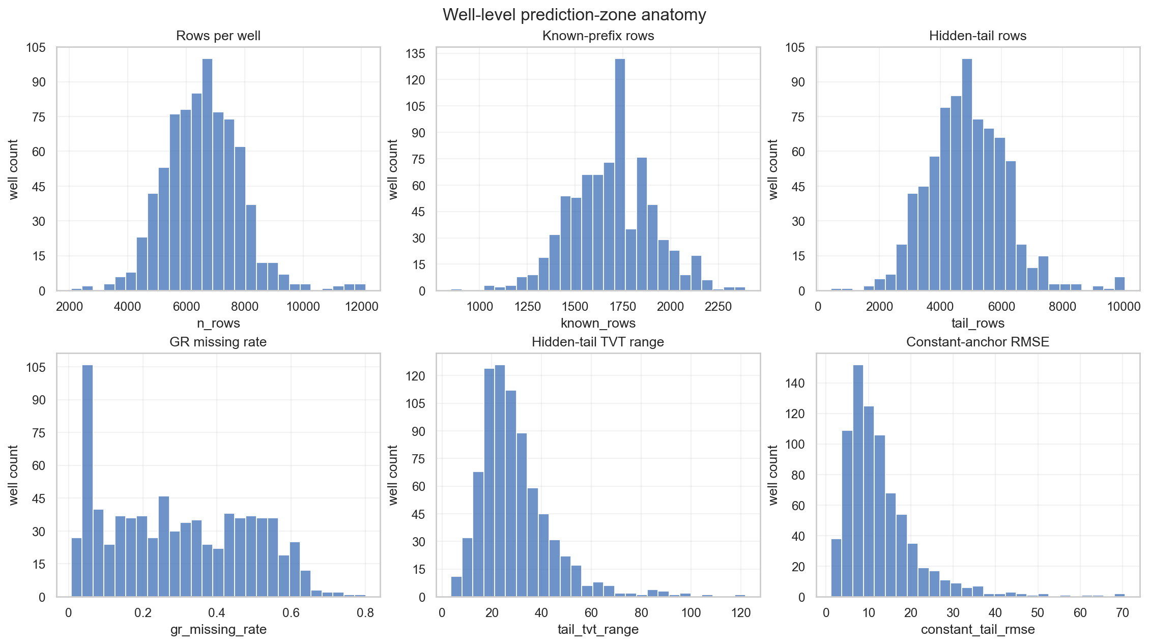
constant-anchor baseline은 다음과 같다.

\[\hat T_{w,i}^{const}=T^{input}_{w,L(w)},\qquad i\in\mathcal H_w.\]

이 단순 baseline은 의외로 강하다. horizontal well은 목표 지층을 따라가도록 뚫리기 때문에, 많은 well에서 TVT가 거의 flat하게 유지된다. 하지만 이 baseline은 두 종류의 well에서 크게 깨진다.

tail이 길고 실제 TVT가 서서히 drift하는 well
지층 mode가 하나의 bundle만큼 잘못 잡힌 well

row-wise RMSE는 긴 tail을 가진 well의 지속적인 오차에 특히 민감하다.

\[RMSE_{row} = \sqrt{ \frac{1}{\sum_w n_w} \sum_w\sum_{i\in\mathcal H_w}e_{w,i}^2 }.\]

따라서 “well 수로는 80%가 잘 맞는다”는 말과 “MSE에서는 datum miss가 더 크다”는 말은 모순이 아니다. 몇 개의 어려운 well이 아주 긴 tail에 걸쳐 큰 offset을 반복하면, squared error mass는 그쪽으로 몰린다.

4. GR/typewell matching: 바코드일 수 있지만 정답 라벨은 아니다

GR은 이 대회에서 가장 강력한 target-free signal 중 하나다. typewell에는 TVT -> GR reference curve가 있고, horizontal well에는 MD -> GR trace가 있다. 자연스러운 생각은 horizontal GR을 typewell GR에 맞춰서 TVT position을 읽는 것이다.

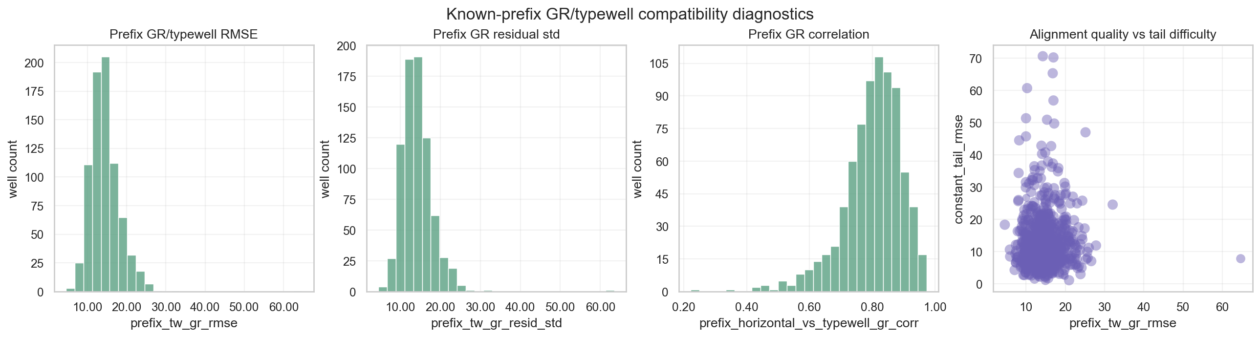
prefix에는 실제 TVT_input이 있으므로, 다음과 같은 prefix consistency check를 만들 수 있다.

\[C_w(\delta) = \left[ \frac{1}{|\mathcal P_w|} \sum_{i\in\mathcal P_w} \left( GR^h_{w,i} - GR^{tw}_w(T^{input}_{w,i}+\delta) \right)^2 \right]^{1/2}.\]

만약 $\delta=0$ 근처에서 cost가 낮으면, prefix GR이 typewell reference와 잘 맞는다는 뜻이다. 하지만 문제는 여기서 끝나지 않는다. cost landscape가 multimodal할 수 있기 때문이다.

GR match는 정답 라벨이 아니라 가능도 신호다. 더 좋은 표현은 argmin 하나가 아니라 posterior-like weight다.

\[q_w(\delta) \propto \exp\{-C_w(\delta)^2/\tau\}.\]

이 관점이 Georgy의 “best GR fit is the wrong depth”와 연결된다. 가장 낮은 GR cost가 실제 TVT datum을 보장하지 않는다. 반복되는 lithology motif가 있으면, GR은 서로 다른 stratigraphic depth에서 비슷하게 맞을 수 있다.

그래서 refork를 계속하는 것보다 더 중요한 일은 cost landscape의 구조를 읽는 것이다.

경우	해석	행동
단일 sharp minimum	datum confidence 높음	단일 경로 또는 강한 correction 가능
경쟁 minima가 가까움	mode ambiguity	posterior mean / hedge
minimum이 prefix anchor와 충돌	calibration 또는 wrong mode 의심	guard / downweight
broad flat landscape	GR evidence 약함	anchor 또는 model stack 쪽으로 후퇴

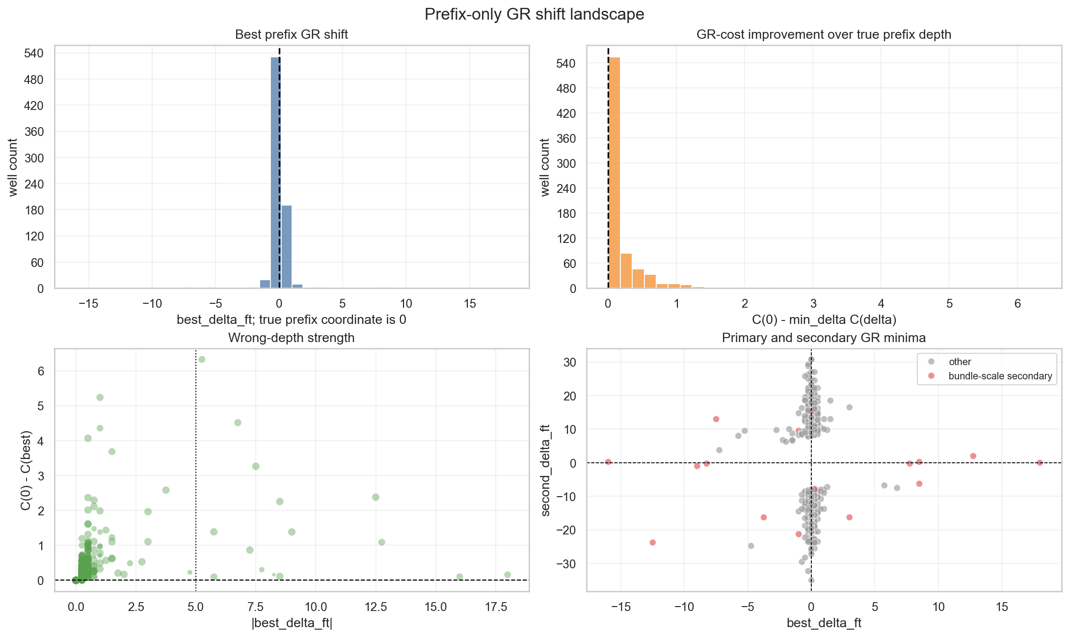
4.1 Notebook snippet: GR shift landscape

GR이 정답 라벨이 아니라 likelihood landscape라는 말은 다음과 같은 scan으로 확인할 수 있다. prefix 구간에서만 여러 vertical shift $\delta$를 시험하고, typewell GR과 horizontal GR의 mismatch를 계산한다.

  
SHIFT_GRID = np.linspace(-40.0, 40.0, 321)

def typewell_gr_at(typewell, tvt):
    tw = typewell[["TVT", "GR"]].dropna().sort_values("TVT")
    return np.interp(tvt, tw["TVT"], tw["GR"])

cost = []
for delta in SHIFT_GRID:
    ref = typewell_gr_at(typewell, prefix["TVT_input"].to_numpy() + delta)
    obs = prefix["GR"].to_numpy()
    cost.append(np.sqrt(np.nanmean((obs - ref) ** 2)))

cost = np.asarray(cost)
best_delta = SHIFT_GRID[np.argmin(cost)]

문제는 best_delta 하나를 고르는 것만으로는 충분하지 않다는 점이다. 더 중요한 값은 최솟값 주변의 모양이다.

\[margin_w=C_{w,(2)}-C_{w,(1)},\qquad q_w(\delta)\propto \exp\{-C_w(\delta)^2/\tau\}.\]

margin이 작거나 $q_w$의 entropy가 크면, 그 well은 하나의 GR minimum으로 단정하기 어렵다. 이때는 “best shift”보다 “mode uncertainty”가 더 중요한 feature가 된다.

5. Georgy의 정정: floor는 하나가 아니다

Georgy의 노트북이 중요했던 이유는 단지 “점수가 좋은 공개 노트북”이어서가 아니다. 오히려 public fork cluster 자체를 의심해야 한다고 말했기 때문이다.

요지는 다음에 가깝다.

carry-last baseline: around 15.9
public fork cluster: around 7.2
public heads: around 5.3-5.5
smooth oracle: around 3

이 숫자들은 하나의 wall을 말하지 않는다. 오히려 여러 종류의 error mass가 층층이 쌓여 있다는 뜻이다.

구간	의미
15.9 -> 9.0	well별 datum/offset을 잡는 효과
9.0 -> 6-7	slope/dip을 읽는 효과
6-7 -> 5.x	wiggle, break, piecewise structure를 더 읽는 효과
5.x -> 3.x	oracle-like smooth shape가 보여주는 남은 ceiling

초기 직관은 “GR fit이 안 되는 곳이 wall이다”에 가까웠다. 하지만 후속 논의 이후 더 정확한 읽기는 다음에 가깝다.

datum은 많은 well에서 합법적인 정보만으로도 상당히 회수 가능하다.
하지만 소수 well의 wrong datum은 MSE를 크게 지배한다.
mode ambiguity는 GR cost margin만으로 단정하기 어렵다.
shape/slope는 실제로 중요한 남은 과제이지만, MSE mass의 전부는 아니다.

이 정정이 이번 노트의 중심축이다.

6. Error anatomy: datum, mode, shape

이 글의 핵심은 error를 하나의 숫자로 보지 않는 것이다.

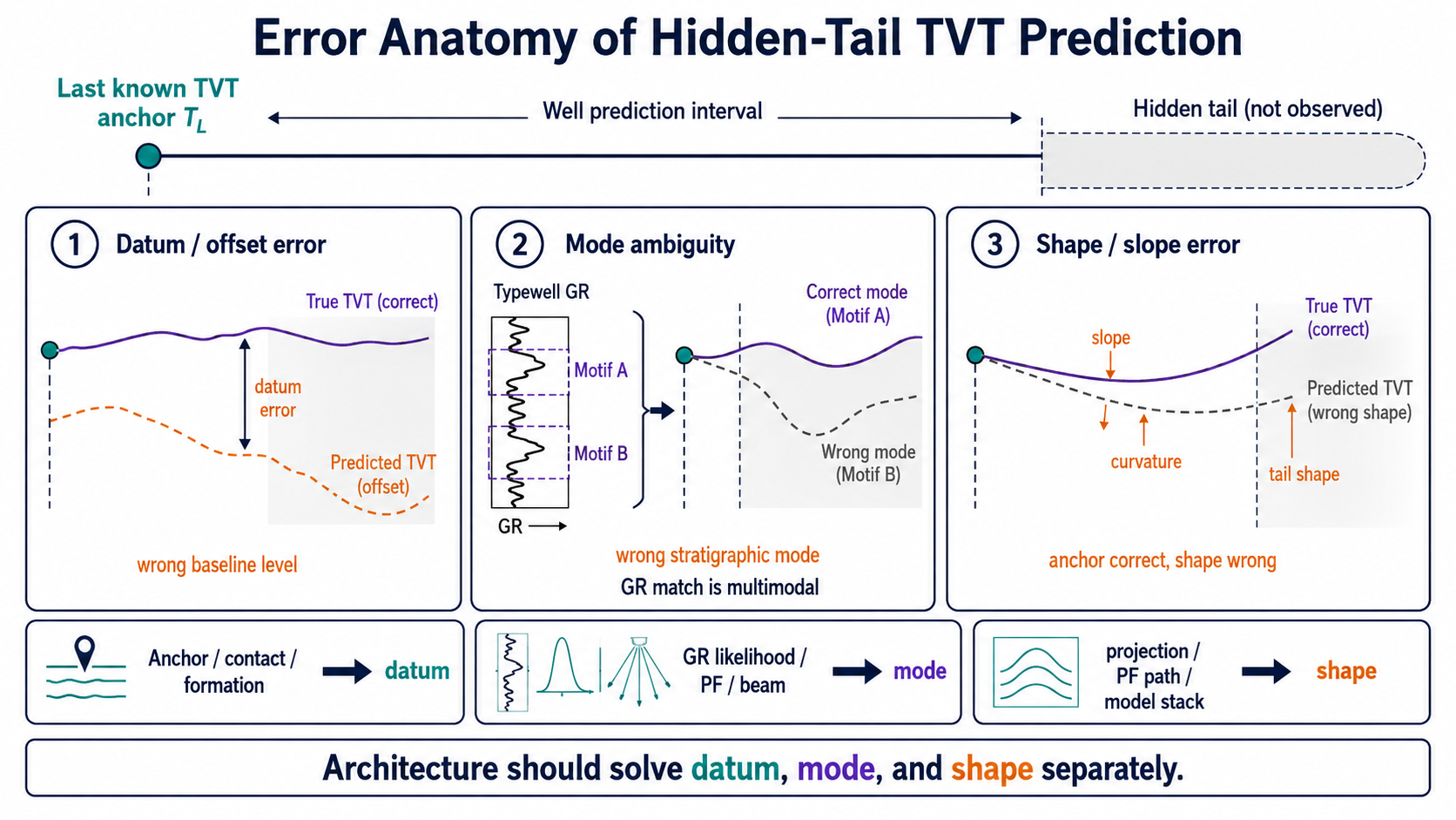
개념적으로 쓰면:

\[T_w(s)-\hat T_w(s) = \underbrace{(D_w-\hat D_w)}_{\text{datum}} + \underbrace{(M_w-\hat M_w)}_{\text{mode}} + \underbrace{(\phi_w(s)-\hat\phi_w(s))}_{\text{shape}}.\]

여기서 $M_w$는 숫자라기보다는 stratigraphic mode 또는 bundle choice를 나타낸다. 이 decomposition은 엄밀한 orthogonal decomposition이라기보다, 각 모델 구성요소가 어떤 책임을 져야 하는지 나누는 지도에 가깝다.

Error component	잘못되면 생기는 현상	대응
datum	tail 전체가 위아래로 밀림	heel calibration, contact, formation prior
mode	비슷한 GR motif 중 잘못된 bundle 선택	GR likelihood, PF/beam, hedge
shape	anchor는 맞지만 slope/curvature가 틀림	projection, path smoothing, residual model

중요한 것은 이 세 가지가 같은 방법으로 해결되지 않는다는 점이다. datum error를 slope model로 고치려 하면 tail 전체가 뒤틀릴 수 있고, mode ambiguity를 hard argmin으로 처리하려 하면 잘못된 bundle에 완전히 고정될 수 있다.

7. MSE split: shape만 남은 것이 아니다

따로 계산한 shape/slope decomposition은 이 논의를 수치화한다.

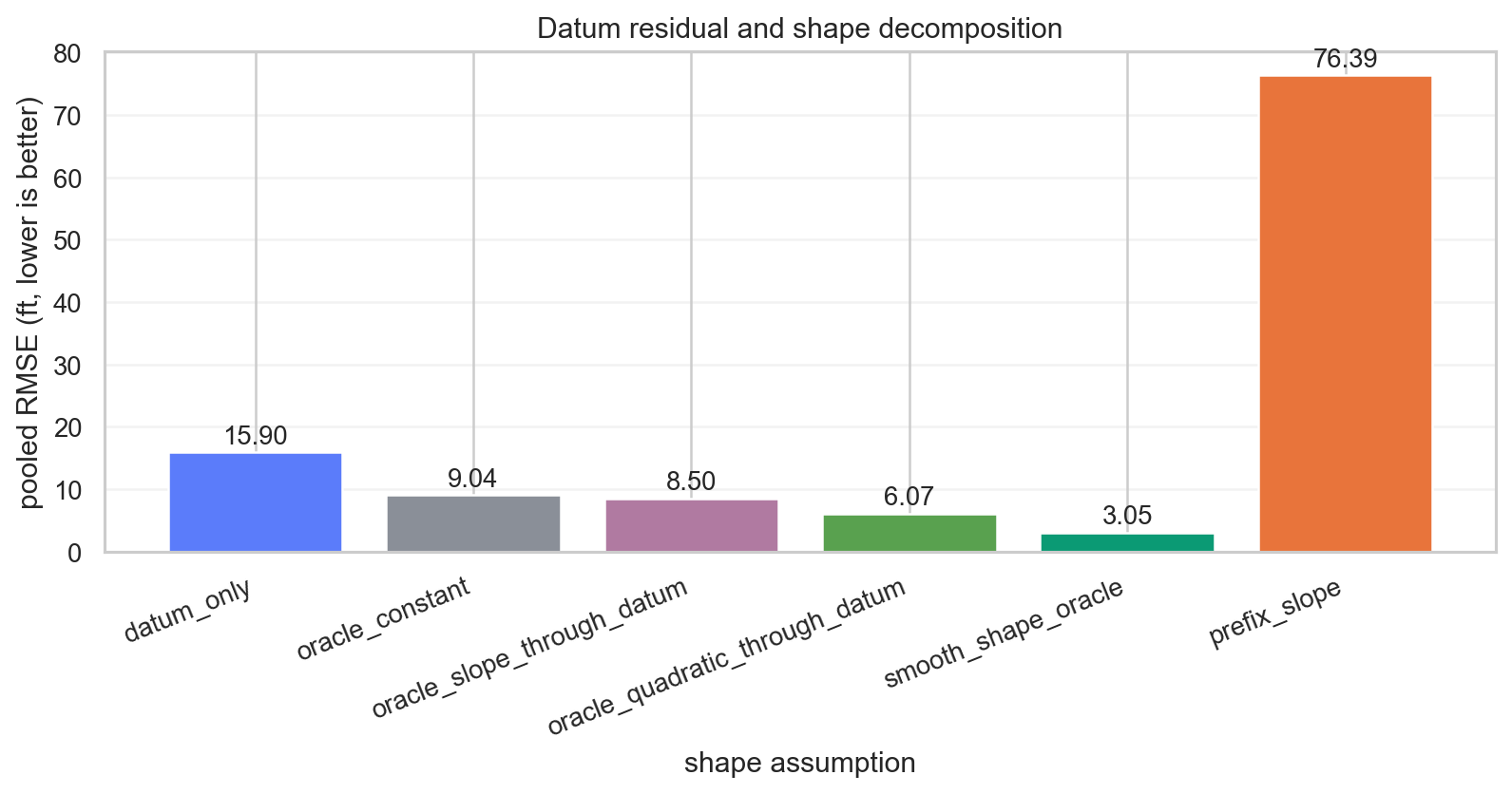
주요 rung은 다음과 같다.

Model	Pooled RMSE
datum only	15.9018
oracle constant	9.0354
prefix slope	76.3878
oracle slope through datum	8.5008
oracle quadratic through datum	6.0717
smooth shape oracle	3.0458

여기서 prefix slope가 매우 나쁘게 나온다는 점이 중요하다. 합법적인 정보만 쓴다고 해서 항상 견고한 것은 아니다. visible heel의 local slope를 tail 전체로 외삽하면, 일부 well에서는 재앙에 가까운 결과가 나온다.

MSE 관점에서는 다음 split이 나온다.

\[MSE_{\text{recoverable}} = RMSE_{\text{datum}}^2 - RMSE_{\text{smooth}}^2.\]

이를 두 부분으로 나누면:

\[MSE_{\text{datum residual}} = RMSE_{\text{datum}}^2 - RMSE_{\text{constant oracle}}^2,\] \[MSE_{\text{pure shape}} = RMSE_{\text{constant oracle}}^2 - RMSE_{\text{smooth oracle}}^2.\]

이번 노트에서 다시 계산한 recoverable MSE는 대략 이렇게 갈라졌다.

Component	Share of recoverable MSE
residual datum miss	70.3%
pure shape	29.7%

이 결과는 “shape가 중요하지 않다”는 뜻이 아니다. 오히려 shape는 상위권 해법이 fork cluster보다 더 내려가기 위해 필요한 신호다. 다만 MSE의 오차량을 기준으로 보면, residual datum miss가 여전히 더 큰 덩어리다. 그래서 “shape is the remaining frontier”라는 단순 문장은 부정확하다. 더 정확한 표현은:

After datum recovery, shape is the modeling frontier,
but residual datum misses still dominate recoverable MSE.

노트북에서는 이 split을 하드코딩하지 않고 RMSE rung에서 직접 계산했다.

  
rmse_datum = ladder.loc["datum_only", "pooled_rmse"]
rmse_const = ladder.loc["oracle_constant", "pooled_rmse"]
rmse_smooth = ladder.loc["smooth_shape_oracle", "pooled_rmse"]

recoverable_mse = rmse_datum**2 - rmse_smooth**2
datum_residual_mse = rmse_datum**2 - rmse_const**2
pure_shape_mse = rmse_const**2 - rmse_smooth**2

datum_share = datum_residual_mse / recoverable_mse
shape_share = pure_shape_mse / recoverable_mse

이 계산이 중요한 이유는, RMSE 차이를 눈으로 비교하면 shape/slope가 더 커 보일 수 있지만, squared error mass로 보면 긴 tail에 반복되는 datum miss가 훨씬 큰 비중을 차지하기 때문이다.

8. Tie wells: 단정 대신 posterior mean

mode ambiguity가 있는 well에서는 두 datum $a$, $b$가 모두 그럴듯할 수 있다. 이때 실제 target이 다음처럼 생겼다고 하자.

\[T\in\{a,b\},\qquad \Pr(T=a)=p.\]

squared loss에서 최적 추정량은 hard argmax가 아니라 posterior mean이다.

\[\hat T = p a + (1-p)b.\]

조건부 분산은 다음과 같다.

\[\operatorname{Var}(T\mid a,b,p)=p(1-p)(a-b)^2.\]

따라서 근거가 mode를 구분하지 못하면 $p\approx 1/2$이고, midpoint hedge가 자연스럽다. 이것이 souldrive의 tie analysis와 연결된다. cost-margin correlation이 $r=+0.054$ 수준이라면, GR cost margin은 mode discriminator로 매우 약하다. 이 경우 한쪽 mode로 단정하는 것은 과신이다.

중요한 뉘앙스는 다음이다.

p is not a magic mode detector.
p is a confidence weight.

즉 $p$가 항상 올바른 mode를 찍어주는 것은 아니다. 다만 ambiguity가 클 때 전부 한쪽에 걸지 않게 만들어준다. public fork cluster에서 보였던 작은 점수 차이도 상당 부분 이 영역에 있었던 것으로 보인다.

왜 midpoint나 posterior mean이 자연스러운지는 squared loss만 봐도 알 수 있다. $p\ge 1/2$라고 해서 항상 $a$로 hard commit하면 기대 손실은:

\[R_{\text{hard}}=(1-p)(a-b)^2.\]

posterior mean $\hat T=pa+(1-p)b$를 쓰면:

\[R_{\text{mean}}=p(1-p)(a-b)^2.\]

둘의 차이는:

\[R_{\text{hard}}-R_{\text{mean}}=(1-p)^2(a-b)^2\ge 0.\]

즉 $p$가 완전히 0 또는 1에 가깝지 않다면, hard decision은 squared loss에서 불필요하게 위험하다. 이것이 tie well에서 hedge가 단순한 요령이 아니라 loss function과 맞는 정책인 이유다.

9. Evidence-to-architecture ladder

최종적으로 이 글이 하려는 말은 “이 feature를 써라”가 아니다. 더 정확히는, 하나의 관찰이 제출 구성요소가 되기까지 거쳐야 하는 사다리를 정리하는 것이다.

한 줄로 쓰면:

\[\text{observation} \rightarrow \text{estimator} \rightarrow \text{validation} \rightarrow \text{profile policy}.\]

예를 들어 GR/typewell landscape는 다음처럼 흘러야 한다.

observed GR/typewell mismatch
-> likelihood surface
-> posterior-like mode weight
-> guarded estimator or hedge
-> profile-specific use

반대로 하면 위험하다. 즉:

public score improves
-> therefore the signal is private-safe

이 결론은 너무 빠르다. public-aggressive policy와 private-safe policy는 분리해야 한다.

10. 세 가지 operating profile

마지막 그림은 이 정책 차이를 요약한다.

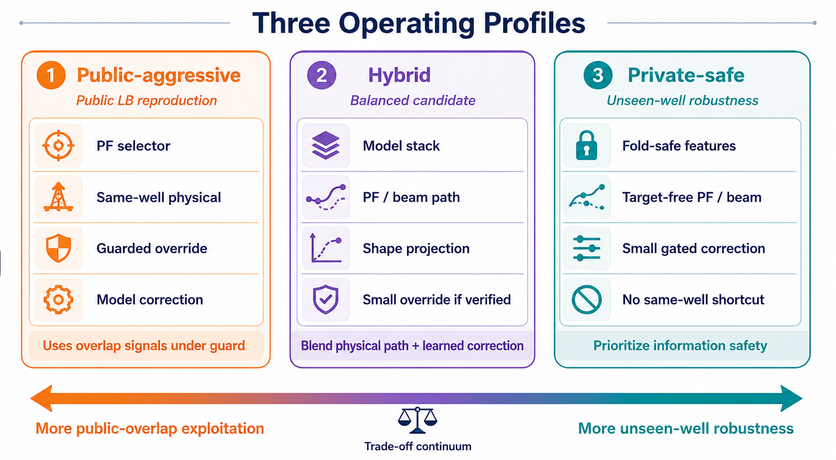
같은 evidence base에서도 세 가지 profile이 나올 수 있다.

Profile	목적	위험
public-aggressive	public LB 재현	overlap signal에 의존할 수 있음
hybrid	path + learned correction의 균형	작은 override도 검증 필요
private-safe	unseen-well robustness	public score는 낮을 수 있음

개념적으로는 다음처럼 쓸 수 있다.

\[\hat T_i^{profile} = \hat T_i^{path} + g_i^{profile}\Delta_i^{model} + h_i^{profile}\Delta_i^{overlap}.\]

private-safe profile에서는 $h_i^{profile}=0$이어야 한다. public-aggressive profile은 $h_i^{profile}>0$를 허용할 수 있지만, 그때는 이것이 private-safe evidence가 아니라 public-overlap exploitation임을 명시해야 한다.

이 구분을 하지 않으면, 노트북에서의 논의는 쉽게 뒤섞인다.

This scores well on public LB.

와

This generalizes to unseen wells.

이 두 문장은 같은 뜻이 아니다.

11. Stop reforking의 실제 의미

이번 노트에서 가장 마음에 드는 문장은 사실 “stop reforking”이다. 이 말은 단순히 public notebook을 베끼지 말라는 도덕적 주장으로 읽히면 안 된다. 더 기술적인 의미가 있다.

If the score difference is inside the stochastic refork band,
it is not yet evidence of a better method.

ROGII에서는 PF, beam, selector, stochastic sampling, public/private overlap, Kaggle execution variance가 모두 섞인다. 같은 코드 또는 거의 같은 코드도 점수가 몇 hundredths, 즉 0.01 단위로 움직일 수 있다. 그러면 7.20과 7.25의 차이가 항상 전략 차이라는 보장은 없다.

따라서 더 나은 질문은 다음이다.

나쁜 질문	좋은 질문
이 fork가 0.03 좋아졌나?	이 변화가 datum/mode/shape 중 무엇을 개선했나?
best GR argmin이 어디인가?	cost landscape가 unimodal인가, bimodal인가?
public score가 올랐나?	private-safe evidence인가, public-overlap policy인가?
CV RMSE가 낮은가?	composed system을 실제 inference path로 검증했는가?

이 노트의 역할은 여기에 있다. leaderboard recipe를 계속 조금씩 바꾸는 것이 아니라, error가 어디에 있는지 보고 다음 실험의 방향을 정하는 것이다.

12. Series 2의 결론

Series 1은 ROGII를 target-free stratigraphic alignment 문제로 재해석했다. Series 2는 그 다음 질문을 다룬다.

Once we agree this is geosteering,
what exactly are we trying to recover?

현재 답은 다음과 같다.

Datum recovery is strong but not perfect.
heel calibration과 typewell alignment로 많은 well의 datum은 회수 가능하다. 하지만 놓친 datum은 tail 전체에 복사되어 MSE를 크게 만든다.
GR argmin is not a label.
반복되는 stratigraphic motif 때문에 best fit이 wrong depth일 수 있다. GR은 likelihood landscape로 읽어야 한다.
Tie wells should be hedged.
hard mode selection evidence가 약할 때 squared loss의 자연스러운 답은 posterior mean이다.
Shape is real but secondary in MSE mass.
slope, curvature, piecewise surface는 상위권 해법으로 가는 데 필요하다. 그러나 recoverable MSE split에서는 residual datum miss가 더 큰 몫을 차지한다.
Validation must be composed.
selector, projection, guard, correction, postprocess를 분리해서 재면 착시가 생긴다. 실제 제출 경로 전체를 평가해야 한다.

그래서 이 작업의 다음 단계는 더 많은 refork가 아니라 더 좋은 decomposition이다.

datum: recover when evidence is strong
mode: hedge when evidence is ambiguous
shape: model only after datum/mode are under control
policy: never confuse public-aggressive with private-safe

이것이 이번 글을 정리한 이유다.

References

ROGII - Wellbore Geology Prediction
ROGII Geological Operations / StarSteer overview
mycarta, ROGII Geosteering Toolkit
Pilkwang Kim, Working Note: Target-Free TVT Geosteering
Georgy Mamarin, Stop reforking: the best GR fit is the wrong depth
Pilkwang Kim, ROGII: Target-Free 지층 대비로 TVT 복원하기 — 데이터 누수 통제 설계
Pilkwang Kim, ROGII: Leakage-Controlled TVT Recovery Through Target-Free Stratigraphic Alignment

AI, Kaggle

This post is licensed under CC BY 4.0 by the author.

ROGII Working Note (2편): Target-Free TVT Geosteering의 오차 해부

대회 배경: 이것은 깊이 예측이 아니라 지층 좌표 복원이다

0. Series 1 이후 달라진 점

1. 왜 tabular regression이 아닌가

2. 정보 경계: 보이는 것과 숨겨진 것

3. Well-level EDA: anchor는 강하지만 완전하지 않다

4. GR/typewell matching: 바코드일 수 있지만 정답 라벨은 아니다

4.1 Notebook snippet: GR shift landscape

5. Georgy의 정정: floor는 하나가 아니다

6. Error anatomy: datum, mode, shape

7. MSE split: shape만 남은 것이 아니다

8. Tie wells: 단정 대신 posterior mean

9. Evidence-to-architecture ladder

10. 세 가지 operating profile

11. Stop reforking의 실제 의미

12. Series 2의 결론

References

Trending Tags