ROGII Working Note (Part 2): Error Anatomy of Target-Free TVT Geosteering

ROGII Working Note (Part 2): Error Anatomy of Target-Free TVT Geosteering

Read Series 1:

• ROGII: Leakage-Controlled TVT Recovery Through Target-Free Stratigraphic Alignment (EN)
• ROGII: Target-Free 지층 대비로 TVT 복원하기 - 데이터 누수 통제 설계 (KR)

Kaggle competition:
ROGII Wellbore Geology Prediction

Kaggle Working Note:
Working Note: Target-Free TVT Geosteering

Korean version:
ROGII Working Note (2편): Target-Free TVT Geosteering의 오차 해부

Critical reference:
Georgy Mamarin - Stop reforking: the best GR fit is the wrong depth

This note owes a lot to the critical discussion in the notebook above. The key correction is simple but important: a low GR matching cost does not automatically mean that we have found the correct TVT depth. That observation helped move the discussion away from score reforking and toward a more useful decomposition of the remaining error.

---

Competition Background: This Is Stratigraphic Coordinate Recovery

The Kaggle task statement says that we need to predict TVT for the evaluation zone of each horizontal well. That sounds simple, but it hides the real structure of the problem. Here, TVT is not just an absolute depth from the surface. It is closer to a stratigraphic coordinate: where the wellbore sits inside the formation column.

That is also how the domain workflow is naturally described. In geosteering, a lateral gamma log is correlated against one or more typewells, often with segmenting, stretching/squeezing, and faulting. In other words, the natural language is not “predict one row at a time.” It is “place a horizontal trajectory inside a typewell coordinate system.”

A row-wise regressor says:

\[\hat T_{w,i}=f(MD_{w,i},X_{w,i},Y_{w,i},Z_{w,i},GR_{w,i}).\]

A geosteering view starts from a well-level coordinate transform:

\[s_i=\frac{MD_i-MD_{start}}{MD_{end}-MD_{start}},\qquad \hat T_w(s_i)=\hat D_w+\hat\phi_w(s_i).\]

Here $\hat D_w$ is the datum: where the well lands in the stratigraphic column. The term $\hat\phi_w$ describes how the tail drifts from that datum. Once this structure is accepted, a good model is no longer just a model with many row features. It is a model that treats datum, mode, and shape as different kinds of evidence.

Everything in this note sits on top of that view.

---

0. What Changed After Series 1

The main point of Series 1 was that ROGII should not be treated as ordinary tabular regression. It is better understood as target-free stratigraphic alignment: recovering a TVT coordinate system without looking at the hidden TVT target.

At that stage, the workflow looked roughly like this:

visible trajectory + GR + typewell + prefix TVT_input
-> target-free pseudo-path
-> residual correction
-> leakage-controlled submission

That framing still holds. But after more public notebooks, discussions, refork experiments, and follow-up analysis, a sharper question emerged:

If the target-free framing is correct,
where does the remaining error actually live?

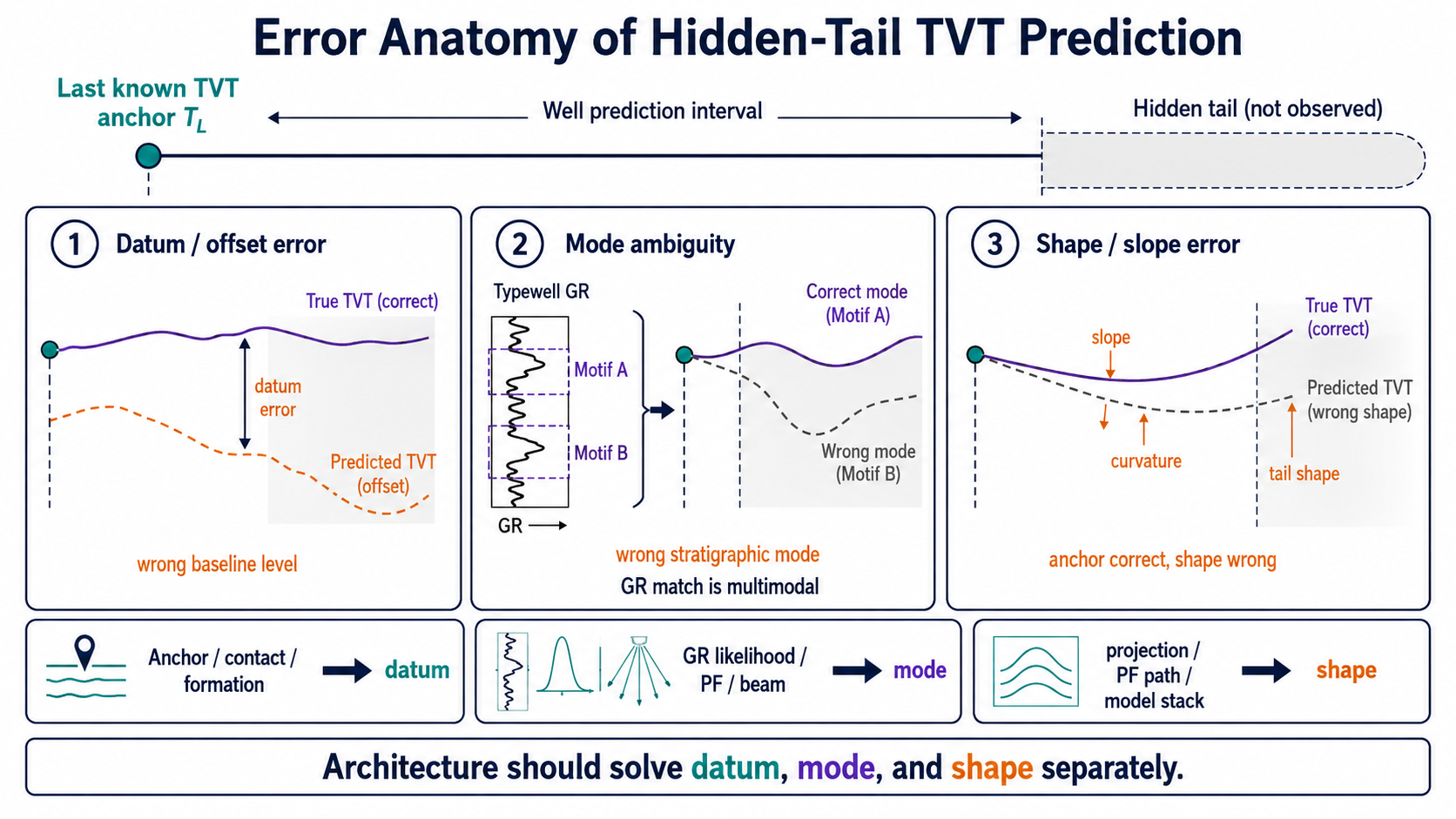
At first, it is tempting to interpret the problem as “find a better GR fit.” Georgy Mamarin’s notebook provides an important correction: the best GR fit is not always the correct TVT depth. A gamma-ray curve behaves like a lithology barcode, but repeated stratigraphic motifs can create plausible matches at multiple depths. The problem is therefore not just choosing the lowest GR cost. It is separating datum error, mode ambiguity, and shape error.

This note revisits the EDA from Series 1 and adds three layers:

Axis	Question	Current reading
datum	At what TVT level does the hidden tail begin?	Recoverable for many wells through prefix and heel calibration, but costly when missed.
mode	Which stratigraphic bundle are we in?	GR cost margin is often too weak for a hard decision; posterior-mean hedging is more natural.
shape	After datum is fixed, how do slope and curvature continue?	Real and important, but smaller than residual datum miss in recoverable MSE mass.

This is not another final submission recipe. It is almost the opposite: a note about stopping score reforks and asking which errors are recoverable, which ones should be hedged, and which ones should be left to a more structured model.

---

1. Why This Is Not Just Tabular Regression

The target column in ROGII is TVT. At first glance, one might feed row-level features such as MD, X, Y, Z, and GR into a row-wise regressor.

But each row is not an independent sample. It is a point along a horizontal well trajectory. The prediction target is not just a scalar per row; it is closer to the entire hidden-tail TVT path of a well.

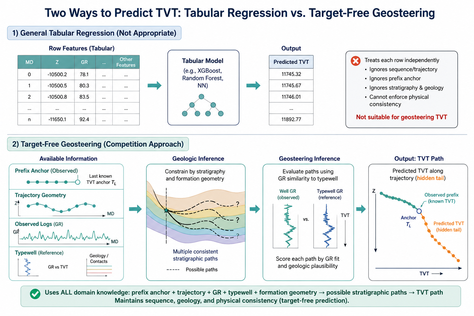
A row model answers:

\[\hat T_{w,i}=f(x_{w,i}).\]

Target-free geosteering estimates a hidden-tail function at the well level:

\[\hat T_w(s)=\hat D_w+\hat\phi_w(s),\qquad s\in[0,1].\]

Here, $\hat D_w$ is the well-level datum and $\hat\phi_w(s)$ is the tail shape. The important point is that the evidence supporting these two terms is not the same.

Component	Main evidence
datum	prefix TVT_input, heel calibration, contact or formation prior
mode	GR/typewell likelihood landscape, PF/beam path, competing minima
shape	trajectory, Z, formation surface, low-order projection, residual model

So the model is not a single black-box regressor. It is a path-estimation system that combines several kinds of evidence. A row-wise model can still be useful, but it should be one component inside the larger path system.

---

2. The Information Boundary: Visible vs Hidden

The central issue in Series 1 was the leakage boundary. The same boundary remains the starting point here.

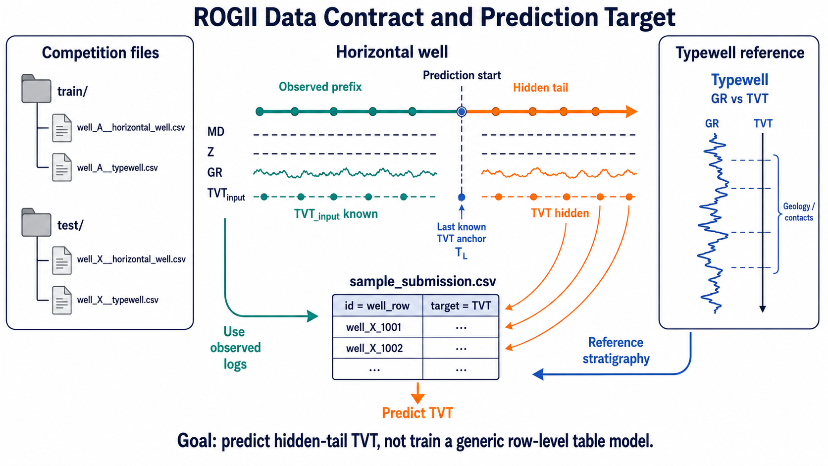
For each well $w$, the observed prefix and hidden tail can be written as:

\[\mathcal P_w=\{i:T^{input}_{w,i}\ \text{is observed}\},\qquad \mathcal H_w=\{i:T^{input}_{w,i}\ \text{is missing}\}.\]

The submitted rows are the hidden-tail rows $\mathcal H_w$. A valid estimator may use:

\[\hat T_{w,\mathcal H} =F\left( X_{w,\mathcal P\cup\mathcal H}, T^{input}_{w,\mathcal P}, \text{typewell}_w \right).\]

Here $X$ is the observed covariate trace, such as MD/X/Y/Z/GR. The full covariate trace is available in the Kaggle input, so it can be used in the batch setting. What is forbidden is the hidden target $T_{w,\mathcal H}$ itself, or statistics fitted from that hidden target.

This distinction matters:

Signal	Usable?	Why
full horizontal GR trace	yes	observed covariate in the test file
typewell GR-vs-TVT curve	yes	reference curve
prefix TVT_input	yes	visible anchor
hidden-tail TVT	no	target
hidden-tail target mean / fitted oracle shape	no	derived from target
train-side oracle ladder	analysis only	ceiling measurement, not an inference feature

A better slogan is not “future GR is leakage.” It is:

Use future observed covariates if they are in the test file.
Do not use future target values, or summaries fitted from them.

In the notebook, this boundary is fixed early at code level. The visible prefix and hidden tail are separated first; the hidden target is used only for analysis or validation.

is_prefix = horizontal["TVT_input"].notna()
prefix = horizontal.loc[is_prefix].copy()
tail = horizontal.loc[~is_prefix].copy()

safe_covariates = ["MD", "X", "Y", "Z", "GR"]
X_full = horizontal[safe_covariates]          # allowed: observed trace
T_prefix = prefix["TVT_input"]               # allowed: visible anchor
T_tail_true = tail["TVT"]                    # analysis / validation only

This small separation matters. Many leakage failures do not come from sophisticated modeling. They come from convenience features that blur this boundary.

---

3. Well-Level EDA: The Anchor Is Strong but Not Perfect

The hidden tail can be long. Even a small datum error is repeated over many rows, so row-wise RMSE can be dominated by a small number of difficult wells.

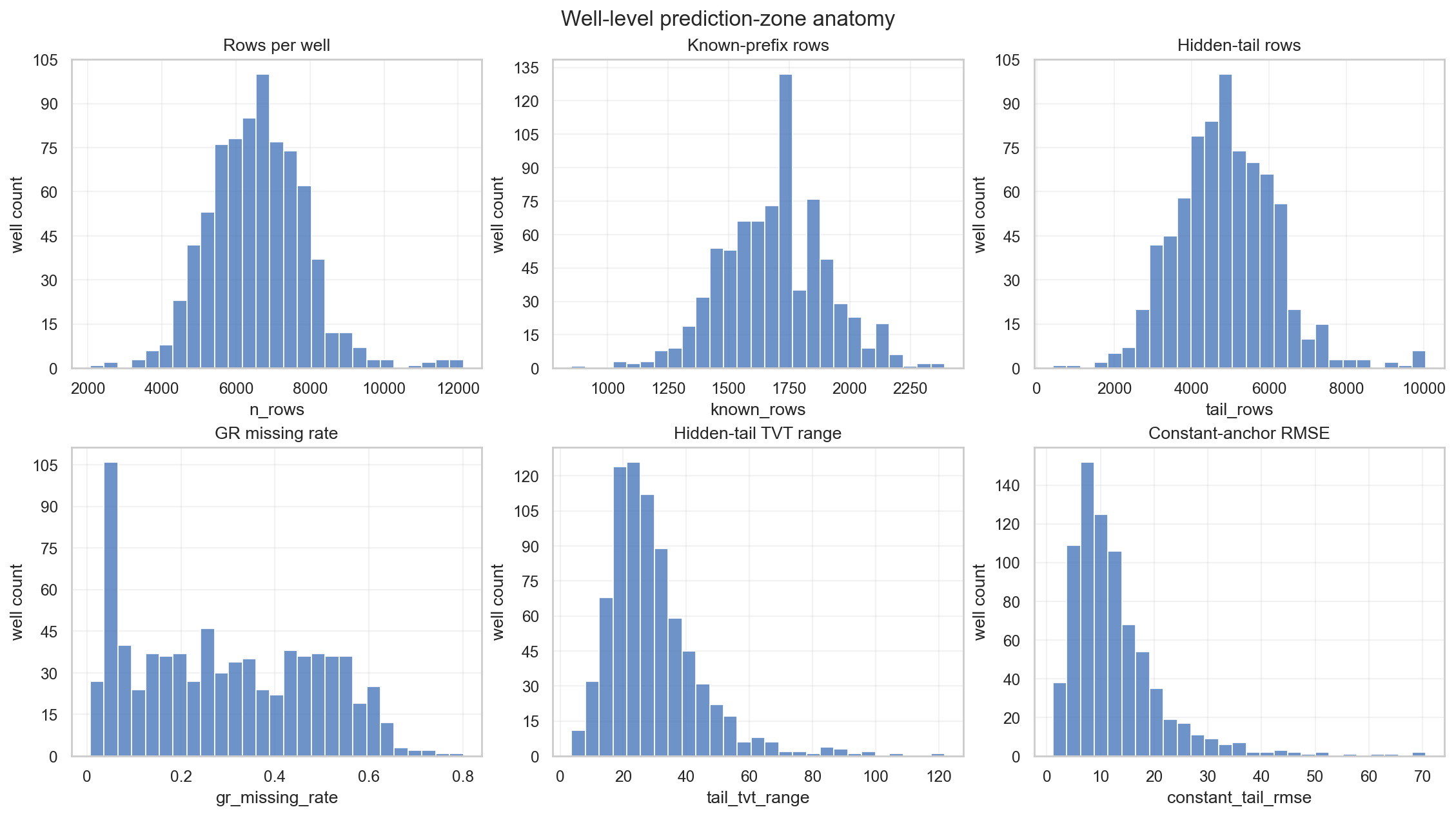
The constant-anchor baseline is:

\[\hat T_{w,i}^{const}=T^{input}_{w,L(w)},\qquad i\in\mathcal H_w.\]

This simple baseline is surprisingly strong. A horizontal well is often drilled to stay within a target formation, so TVT can remain nearly flat for many wells. But the baseline breaks badly in two cases:

1. the hidden tail is long and true TVT drifts gradually;
2. the stratigraphic mode is shifted by one bundle.

Row-wise RMSE is especially sensitive to persistent errors in long tails:

\[RMSE_{row} = \sqrt{ \frac{1}{\sum_w n_w} \sum_w\sum_{i\in\mathcal H_w}e_{w,i}^2 }.\]

So there is no contradiction between “80% of wells are roughly localized” and “residual datum misses dominate MSE.” A few hard wells can replicate a large offset over long tails, and squared error mass then concentrates there.

---

4. GR/Typewell Matching: Barcode, Not Label

GR is one of the strongest target-free signals in this competition. The typewell gives a TVT -> GR reference curve, while the horizontal well gives an MD -> GR trace. A natural idea is to align horizontal GR to typewell GR and read off TVT position.

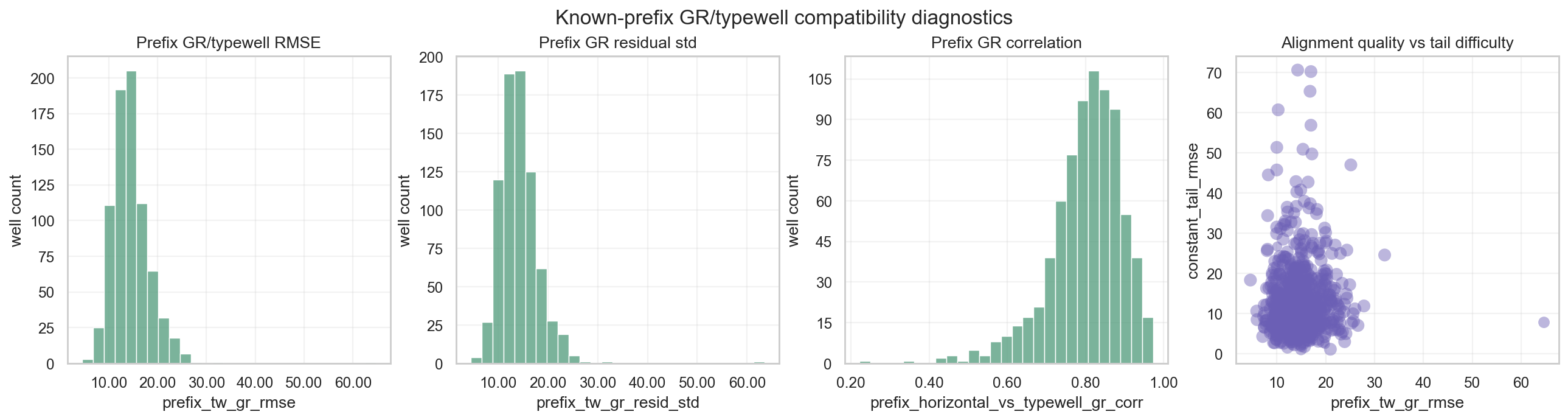
Because the prefix has true TVT_input, we can define a prefix consistency cost:

\[C_w(\delta) = \left[ \frac{1}{|\mathcal P_w|} \sum_{i\in\mathcal P_w} \left( GR^h_{w,i} - GR^{tw}_w(T^{input}_{w,i}+\delta) \right)^2 \right]^{1/2}.\]

If the cost is low near $\delta=0$, the prefix GR is consistent with the typewell reference. But that is not the end of the problem, because the cost landscape can be multimodal.

GR matching is not a label. It is a likelihood signal. A better representation is not a single argmin, but a posterior-like weight:

\[q_w(\delta) \propto \exp\{-C_w(\delta)^2/\tau\}.\]

This is where Georgy’s “the best GR fit is the wrong depth” matters. A repeated lithology motif can create similar GR costs at different stratigraphic depths. The lowest cost does not guarantee the correct TVT datum.

So the useful task is not to keep reforking a single argmin rule. It is to read the structure of the landscape:

Case	Interpretation	Action
one sharp minimum	high datum confidence	single path or strong correction
competing minima close together	mode ambiguity	posterior mean / hedge
minimum conflicts with prefix anchor	calibration or wrong mode suspected	guard / downweight
broad flat landscape	weak GR evidence	retreat to anchor or model stack

---

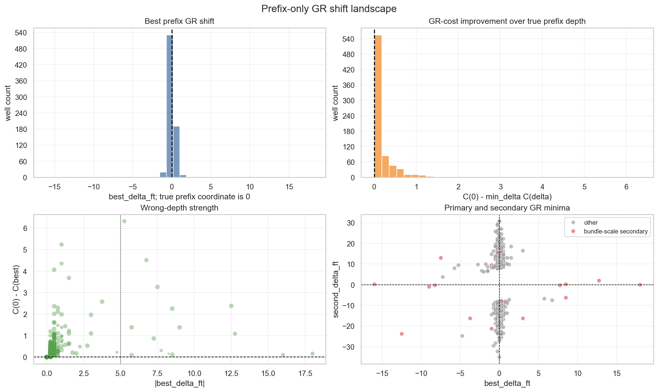
4.1 Notebook Snippet: GR Shift Landscape

The claim that GR is a likelihood landscape rather than a label can be checked with a simple prefix-only shift scan. We try a grid of vertical shifts $\delta$ and compute the mismatch between horizontal GR and typewell GR over the visible prefix.

SHIFT_GRID = np.linspace(-40.0, 40.0, 321)

def typewell_gr_at(typewell, tvt):
    tw = typewell[["TVT", "GR"]].dropna().sort_values("TVT")
    return np.interp(tvt, tw["TVT"], tw["GR"])

cost = []
for delta in SHIFT_GRID:
    ref = typewell_gr_at(typewell, prefix["TVT_input"].to_numpy() + delta)
    obs = prefix["GR"].to_numpy()
    cost.append(np.sqrt(np.nanmean((obs - ref) ** 2)))

cost = np.asarray(cost)
best_delta = SHIFT_GRID[np.argmin(cost)]

The problem is that best_delta alone is not enough. The shape around the minimum carries the more important information:

\[margin_w=C_{w,(2)}-C_{w,(1)},\qquad q_w(\delta)\propto \exp\{-C_w(\delta)^2/\tau\}.\]

If the margin is small, or if the entropy of $q_w$ is large, the well is not safely localized by one GR minimum. In that case, mode uncertainty is more important than the best shift itself.

---

5. Georgy’s Correction: There Is Not One Floor

Georgy’s notebook was important not merely because it was a strong public notebook. It was important because it questioned the public fork cluster itself.

The rough ladder is:

carry-last baseline: around 15.9
public fork cluster: around 7.2
public heads: around 5.3-5.5
smooth oracle: around 3

These numbers do not indicate one wall. They indicate multiple layers of error mass.

Interval	Meaning
15.9 -> 9.0	effect of fixing well-level datum / offset
9.0 -> 6-7	effect of reading slope / dip
6-7 -> 5.x	effect of wiggle, break, and piecewise structure
5.x -> 3.x	remaining ceiling suggested by oracle-like smooth shape

The initial intuition was close to “GR fit failure is the wall.” The later reading is more precise:

1. datum is recoverable for many wells using legal evidence;
2. a small number of wrong-datum wells dominate MSE;
3. mode ambiguity is hard to resolve from GR cost margin alone;
4. shape and slope remain important, but they are not the whole remaining MSE mass.

This correction is the backbone of the note.

---

6. Error Anatomy: Datum, Mode, Shape

The core idea is to stop treating error as one number.

Conceptually:

\[T_w(s)-\hat T_w(s) = \underbrace{(D_w-\hat D_w)}_{\text{datum}} + \underbrace{(M_w-\hat M_w)}_{\text{mode}} + \underbrace{(\phi_w(s)-\hat\phi_w(s))}_{\text{shape}}.\]

Here $M_w$ is less a scalar than a stratigraphic mode or bundle choice. This is not meant as a rigorous orthogonal decomposition. It is a map of responsibilities: which part of the system should handle which kind of error?

Error component	Failure mode	Response
datum	the entire tail shifts up or down	heel calibration, contact, formation prior
mode	the model chooses the wrong repeated GR motif	GR likelihood, PF/beam, hedge
shape	anchor is right, but slope or curvature is wrong	projection, path smoothing, residual model

The important point is that these errors are not fixed by the same mechanism. Trying to fix datum error with a slope model can distort the whole tail. Treating mode ambiguity as a hard argmin can lock the estimator into the wrong bundle.

---

7. MSE Split: Shape Is Not the Only Thing Left

The shape/slope decomposition quantifies the previous section.

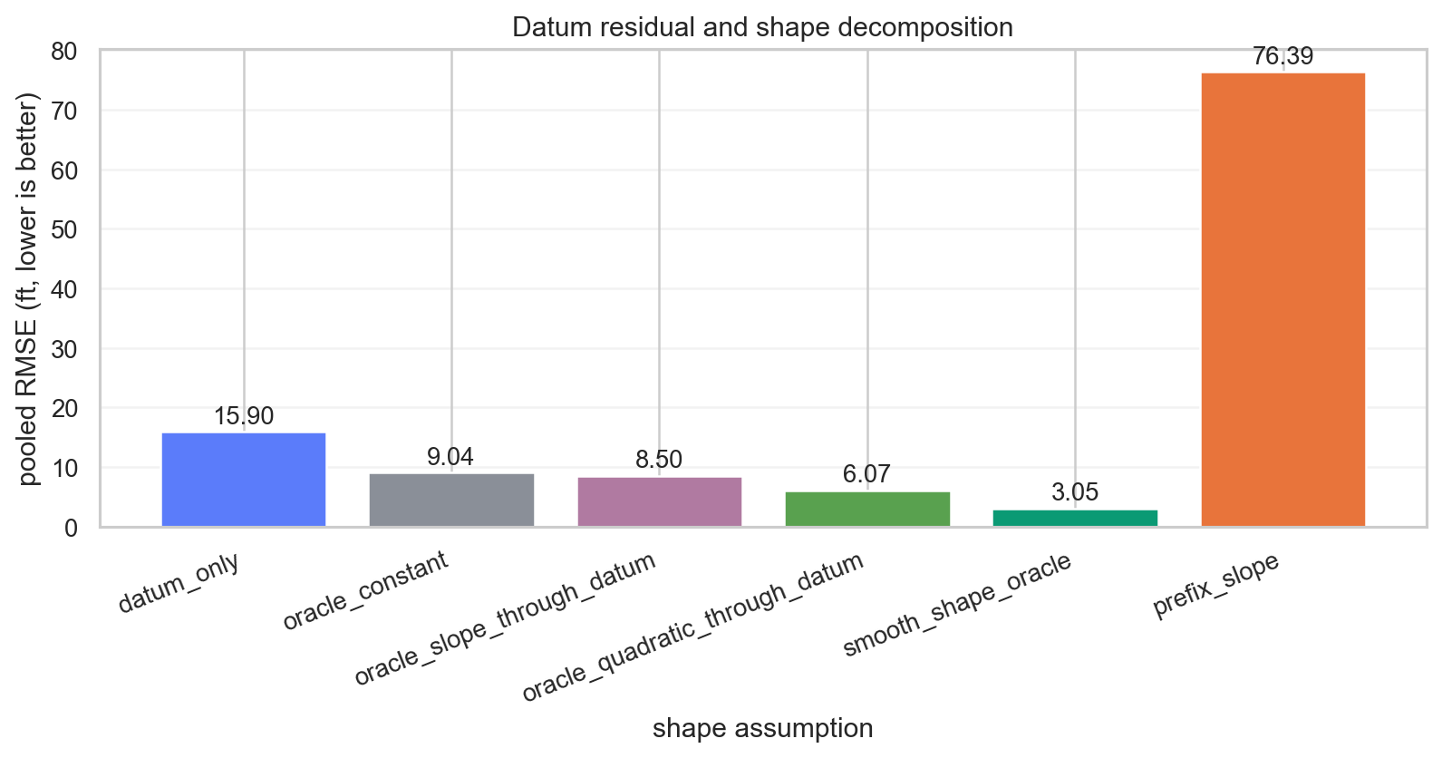
The main rungs are:

Model	Pooled RMSE
datum only	15.9018
oracle constant	9.0354
prefix slope	76.3878
oracle slope through datum	8.5008
oracle quadratic through datum	6.0717
smooth shape oracle	3.0458

The disastrous prefix-slope result is important. A legal signal is not automatically a robust signal. Extrapolating the local heel slope through the full tail can fail catastrophically on some wells.

In MSE terms:

\[MSE_{\text{recoverable}} = RMSE_{\text{datum}}^2 - RMSE_{\text{smooth}}^2.\]

Split this into two pieces:

\[MSE_{\text{datum residual}} = RMSE_{\text{datum}}^2 - RMSE_{\text{constant oracle}}^2,\] \[MSE_{\text{pure shape}} = RMSE_{\text{constant oracle}}^2 - RMSE_{\text{smooth oracle}}^2.\]

The recomputed recoverable-MSE split is roughly:

Component	Share of recoverable MSE
residual datum miss	70.3%
pure shape	29.7%

This does not mean shape is unimportant. Shape is one of the signals needed to move below the public fork cluster. But by error mass, residual datum miss is still the larger component. So the simple statement “shape is the remaining frontier” is incomplete. A more accurate statement is:

After datum recovery, shape is the modeling frontier,
but residual datum misses still dominate recoverable MSE.

The notebook computes this split directly from the RMSE ladder rather than hard-coding the percentages:

rmse_datum = ladder.loc["datum_only", "pooled_rmse"]
rmse_const = ladder.loc["oracle_constant", "pooled_rmse"]
rmse_smooth = ladder.loc["smooth_shape_oracle", "pooled_rmse"]

recoverable_mse = rmse_datum**2 - rmse_smooth**2
datum_residual_mse = rmse_datum**2 - rmse_const**2
pure_shape_mse = rmse_const**2 - rmse_smooth**2

datum_share = datum_residual_mse / recoverable_mse
shape_share = pure_shape_mse / recoverable_mse

This matters because RMSE differences can visually overemphasize the shape/slope ladder. In squared-error mass, a missed datum copied through a long tail is much more expensive.

---

8. Tie Wells: Use Posterior Mean, Not Overconfident Decisions

For some wells, two datums $a$ and $b$ can both be plausible. Suppose:

\[T\in\{a,b\},\qquad \Pr(T=a)=p.\]

Under squared loss, the optimal estimate is not the hard argmax. It is the posterior mean:

\[\hat T = p a + (1-p)b.\]

The conditional variance is:

\[\operatorname{Var}(T\mid a,b,p)=p(1-p)(a-b)^2.\]

If the evidence cannot distinguish the mode, then $p\approx 1/2$, and a midpoint hedge is natural. This connects to souldrive’s tie analysis: if the cost-margin correlation is only about $r=+0.054$, then the GR cost margin is a very weak discriminator. A hard choice in that situation is overconfidence.

The nuance is:

p is not a magic mode detector.
p is a confidence weight.

That is, $p$ does not always pick the correct mode. It prevents the estimator from betting everything on one mode when the evidence is ambiguous. A meaningful part of the small public fork differences probably lived in this zone.

The squared-loss reason is straightforward. If $p\ge 1/2$ and we always hard-commit to $a$, the expected loss is:

\[R_{\text{hard}}=(1-p)(a-b)^2.\]

If we use the posterior mean $\hat T=pa+(1-p)b$, the expected loss is:

\[R_{\text{mean}}=p(1-p)(a-b)^2.\]

The improvement is:

\[R_{\text{hard}}-R_{\text{mean}}=(1-p)^2(a-b)^2\ge 0.\]

So unless $p$ is already very close to 0 or 1, a hard decision is unnecessarily risky under squared loss. This is why hedging tie wells is not just a leaderboard trick; it matches the loss function.

---

9. Evidence-to-Architecture Ladder

The conclusion is not “use this feature.” The better conclusion is that an observation should pass through a ladder before it becomes a submission component.

In one line:

\[\text{observation} \rightarrow \text{estimator} \rightarrow \text{validation} \rightarrow \text{profile policy}.\]

For example, a GR/typewell landscape should flow like:

observed GR/typewell mismatch
-> likelihood surface
-> posterior-like mode weight
-> guarded estimator or hedge
-> profile-specific use

The reverse direction is dangerous:

public score improves
-> therefore the signal is private-safe

That inference is too fast. A public-aggressive policy and a private-safe policy should be separated.

---

10. Three Operating Profiles

The final figure summarizes this policy distinction.

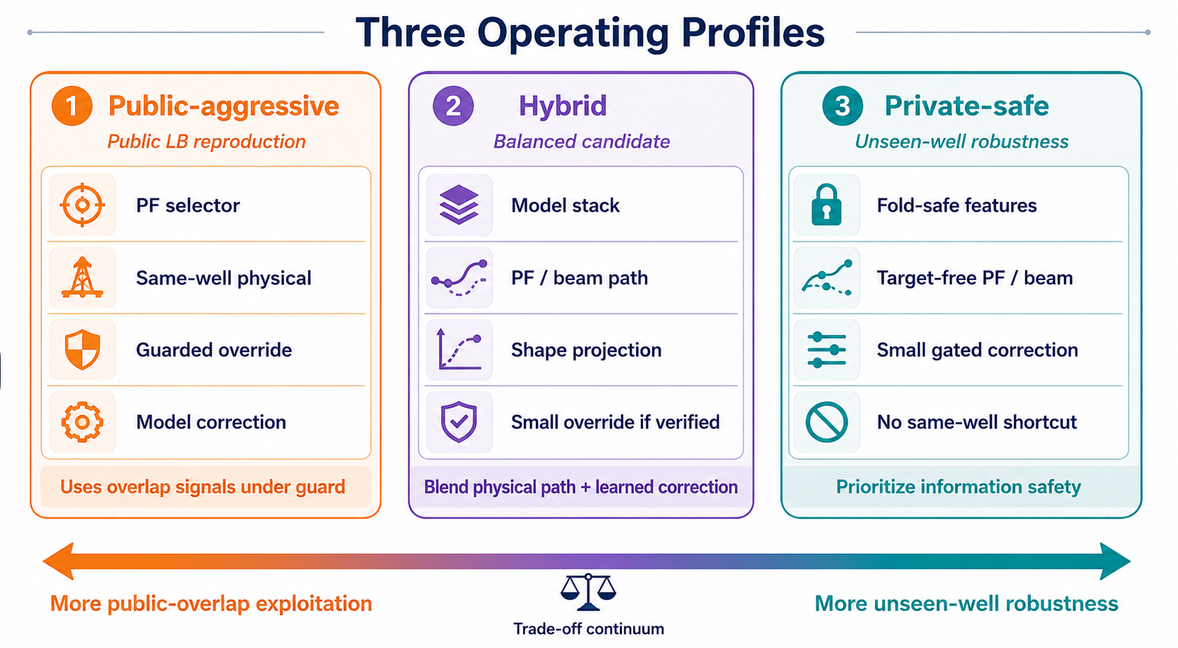
The same evidence base can lead to three different profiles:

Profile	Goal	Risk
public-aggressive	reproduce public LB behavior	may depend on overlap signal
hybrid	balance path and learned correction	even small overrides need validation
private-safe	unseen-well robustness	public score can be lower

Conceptually:

\[\hat T_i^{profile} = \hat T_i^{path} + g_i^{profile}\Delta_i^{model} + h_i^{profile}\Delta_i^{overlap}.\]

For a private-safe profile, $h_i^{profile}=0$. A public-aggressive profile may allow $h_i^{profile}>0$, but then it should be described as public-overlap exploitation, not private-safe evidence.

Without this distinction, notebook discussions easily blur two different claims:

This scores well on public LB.

and

This generalizes to unseen wells.

These are not the same claim.

---

11. What “Stop Reforking” Really Means

The phrase I like most from this line of discussion is “stop reforking.” This is not merely a moral claim about not copying public notebooks. It has a technical meaning:

If the score difference is inside the stochastic refork band,
it is not yet evidence of a better method.

In ROGII, PF, beam search, selector logic, stochastic sampling, public/private overlap, and Kaggle execution variance all interact. The same code, or almost the same code, can move by a few hundredths. A difference between 7.20 and 7.25 is not always a strategy difference.

The better questions are:

Weak question	Better question
Did this fork improve by 0.03?	Which component did it improve: datum, mode, or shape?
Where is the best GR argmin?	Is the cost landscape unimodal or bimodal?
Did public score improve?	Is this private-safe evidence or public-overlap policy?
Is CV RMSE lower?	Was the composed inference path evaluated end to end?

That is the role of this note: not to keep tweaking leaderboard recipes, but to locate the error and decide what kind of experiment should come next.

---

12. Series 2 Takeaways

Series 1 reframed ROGII as target-free stratigraphic alignment. Series 2 asks the next question:

Once we agree this is geosteering,
what exactly are we trying to recover?

The current answer is:

1. Datum recovery is strong but not perfect.
   Heel calibration and typewell alignment recover the datum for many wells. Missed datum is copied through the tail and becomes expensive in MSE.

2. GR argmin is not a label.
   Repeated stratigraphic motifs can make the best fit land at the wrong depth. GR should be read as a likelihood landscape.

3. Tie wells should be hedged.
   When hard mode-selection evidence is weak, the squared-loss answer is the posterior mean.

4. Shape is real but secondary in MSE mass.
   Slope, curvature, and piecewise surfaces matter for top solutions. But in the recoverable-MSE split, residual datum miss is the larger part.

5. Validation must be composed.
   Measuring selector, projection, guard, correction, and postprocessing in isolation can be misleading. The complete inference path should be evaluated.

The next step is not more reforking. It is better decomposition:

datum: recover when evidence is strong
mode: hedge when evidence is ambiguous
shape: model only after datum/mode are under control
policy: never confuse public-aggressive with private-safe

That is why I wanted to write this note.

---

References

• ROGII - Wellbore Geology Prediction
• ROGII Geological Operations / StarSteer overview
• mycarta, ROGII Geosteering Toolkit
• Pilkwang Kim, Working Note: Target-Free TVT Geosteering
• Georgy Mamarin, Stop reforking: the best GR fit is the wrong depth
• Pilkwang Kim, ROGII: Leakage-Controlled TVT Recovery Through Target-Free Stratigraphic Alignment
• Pilkwang Kim, ROGII: Target-Free 지층 대비로 TVT 복원하기 - 데이터 누수 통제 설계