ROGII: Leakage-Controlled TVT Recovery Through Target-Free Stratigraphic Alignment

ROGII: Leakage-Controlled TVT Recovery Through Target-Free Stratigraphic Alignment

Competition link:
ROGII Wellbore Geology Prediction

Kaggle code:
ROGII EDA: Target-Free Alignment for TVT

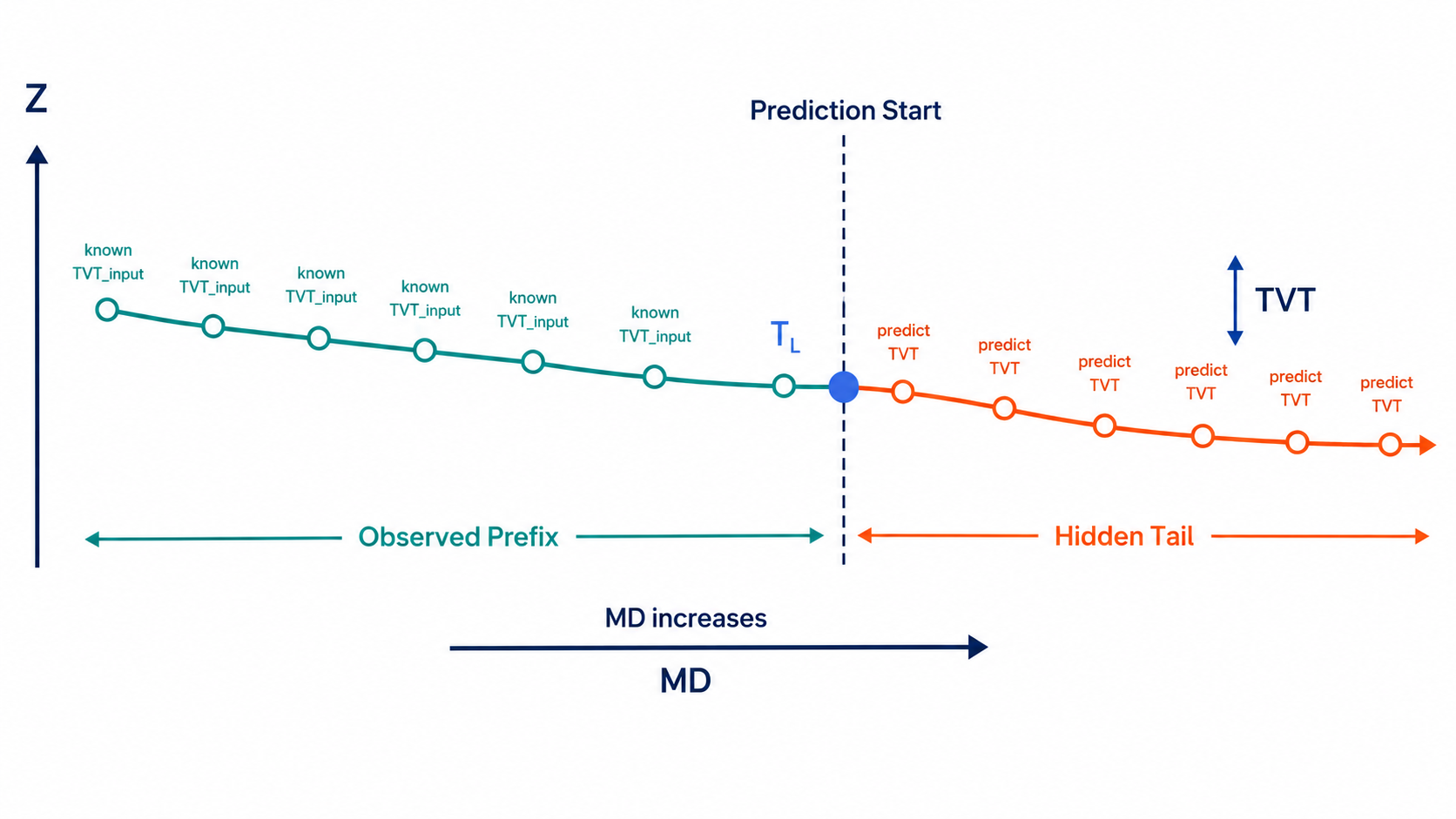
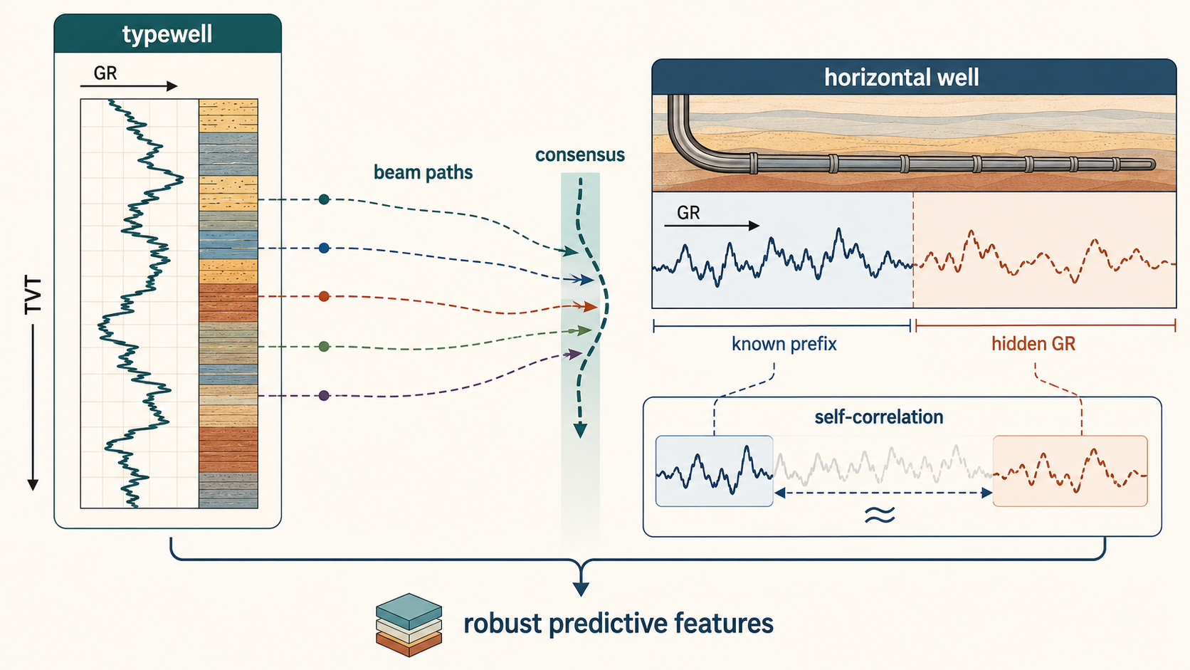
The target is TVT, true vertical thickness, along the hidden tail of a horizontal well.
For each test well, the first prefix has known TVT_input; the long remaining interval must be predicted from measured geometry and gamma-ray evidence.

The rows are not independent samples in the usual tabular sense. Each row is a point on a drilled trajectory. MD increases along the well path, while X/Y/Z describe where that point sits in space. In a horizontal well, the drilled path can travel thousands of feet laterally while changing vertical position much more slowly. The prediction target, TVT, is a stratigraphic coordinate: it describes where the well is relative to geological layers, not merely how deep the row is along the drill path.

The basic vocabulary is:

Term	Meaning In This Problem
MD	Measured depth along the wellbore path. It increases with drilled distance.
X/Y/Z	Spatial coordinates of the wellbore point. Z carries vertical position.
TVD	True vertical depth, a vertical depth coordinate rather than a path length.
TVT	True vertical thickness coordinate used to place the well relative to the geological section.
GR	Gamma-ray log. It measures natural radioactivity and often changes with lithology and shale content.
Typewell	A vertical reference well where TVT -> GR is known.
Horizontal well	The target well where the prefix has known TVT_input, but the hidden tail needs TVT recovery.

This creates an unusual inverse problem:

typewell:
    TVT -> GR reference curve

horizontal well:
    MD/X/Y/Z -> GR observed curve

goal:
    MD/X/Y/Z/GR -> TVT hidden curve

The apparent regression target is one column, but the physical object is a curve. A row-level model that sees only local numeric columns has to rediscover three facts at once: where the well sits in the formation, how the GR pattern aligns to the typewell, and how much of the prefix anchor should remain trusted as the tail gets longer.

The central difficulty is not simply regression. It is recovering a stratigraphic coordinate under a strict information boundary:

Known at prediction time:
MD, X, Y, Z, GR, prefix TVT_input

Hidden:
tail TVT

Useful but dangerous:
same-well train/test overlap, formation tops, full-tail covariate paths, OOF artifacts

The information boundary reduces to one rule:

Use every target-free geological signal, but never smuggle hidden-tail TVT into validation or inference.

target-free does not mean weak or blind. It means the estimator can use full covariate geometry, GR traces, typewell curves, prefix calibration, and train-fold spatial geology, but cannot use the hidden tail labels or any statistic derived from them. In this setting, a strong feature can be a whole predicted path produced from physics or stratigraphic alignment, not a scalar column.

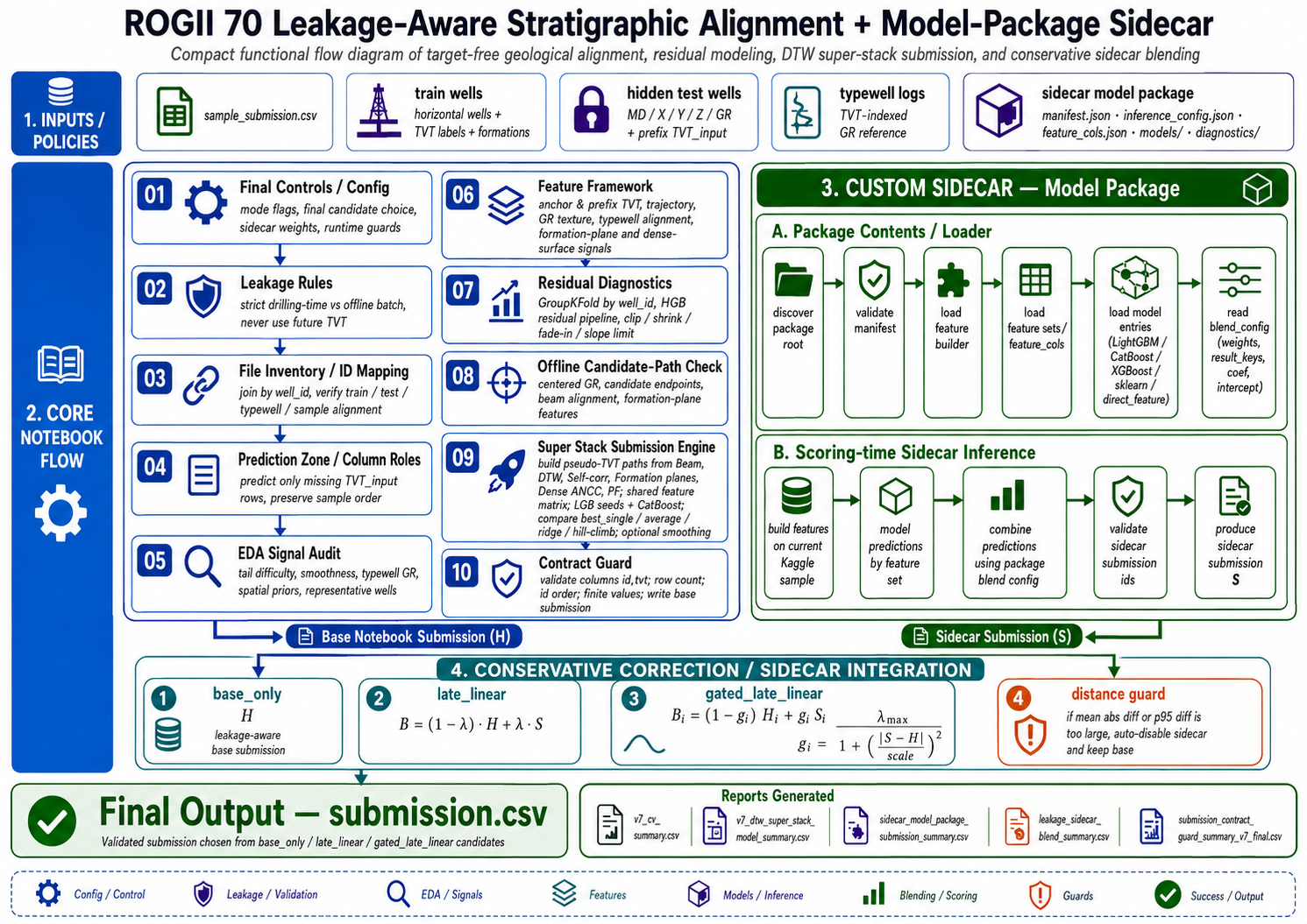
The major layers are:

Layer	Role
Prefix anchor	Use the last known TVT_input as a strong local origin.
Geometry	Convert X/Y/Z/MD movement into drift, slope, curvature, and formation-relative features.
GR barcode	Align horizontal GR traces to typewell GR traces without using tail labels.
Formation model	Estimate structural surfaces from safe spatial information.
PF / beam / DTW paths	Generate target-free pseudo-TVT trajectories.
Residual GBDT / stack	Learn when each physical estimate is reliable.
Contract guard	Emit exactly id,tvt in sample order with finite values.

The dependency direction is:

observed covariates
-> target-free geological hypotheses
-> reliability features
-> residual correction
-> conservative post-processing

This order keeps the model from using tree depth to invent arbitrary row-wise behavior. The base paths carry geology; the residual model learns when those paths are biased.

The guarded pf_residual_gbdt profile has the following output summary:

Quantity	Value
Train horizontal wells	773
Test horizontal wells	3
Submission rows	14,151
Train hidden-tail rows	3,783,989
PF-only OOF RMSE	11.0106
PF + residual GBDT OOF RMSE	10.5696
Final prediction mean	11906
Final prediction std	277.81
Final prediction range	11601 to 12242

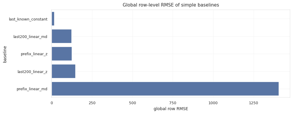
The RMSE gain is modest in absolute size, but it is measured on top of a physically constrained path rather than a naive tabular baseline.

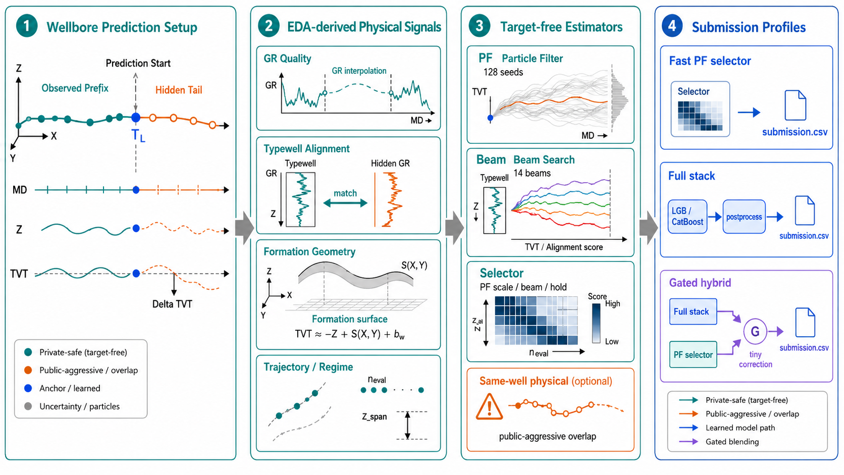
1. Hidden-Tail Geometry

Each well is divided into a known prefix and a hidden tail.
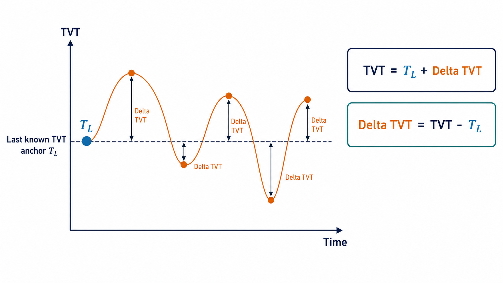
The observed prefix gives a clean local anchor:

\[T_{w,L} = \operatorname{last\_known\_TVT}(w)\]

The regression target is easier to model as an anchored residual:

\[\Delta T_{i} = T_i - T_{w,L}\]

so the final row-level prediction becomes:

\[\hat{T}_{i} = T_{w,L} + \widehat{\Delta T}_{i}\]

The residual form follows from the tail geometry. The tail usually starts close to the last known TVT. A model that immediately drifts too far away from the prefix anchor can lose many rows before the geological signal has enough evidence to justify the move.

The prefix is more than a convenient starting value. It defines a local coordinate system for the well:

Prefix Quantity	Why It Matters
last known TVT_input	Initial stratigraphic position at prediction start.
prefix GR versus typewell GR	Calibration of the GR barcode for the specific well.
prefix slope of TVT versus MD	Local drift direction before the hidden tail.
prefix trajectory slope and curvature	How the borehole was moving into the hidden interval.
prefix residual against formation surfaces	Local structural offset b_w.

The prediction therefore begins from a known geological state rather than from a global mean or from a test-well row index. Every candidate path is judged by how plausibly it evolves from that state.

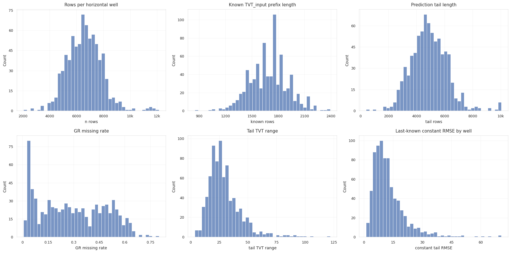
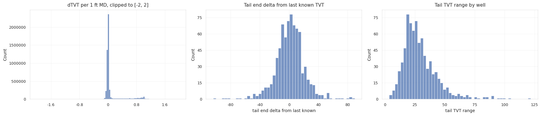
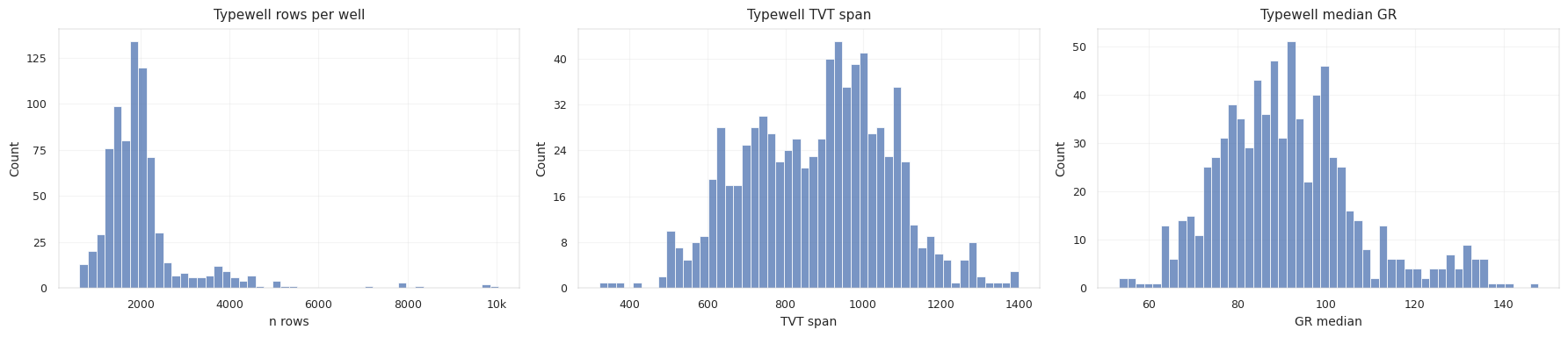
The training wells show a consistent single hidden block after the prefix:

Tail Statistic	Mean	Median	95%	Max
known_rows	1692.5	1703	2053	2392
tail_rows	4895.2	4840	6918	10052
tail_tvt_range	29.41	26.37	54.42	121.84
constant_tail_rmse	12.81	10.67	29.01	70.64

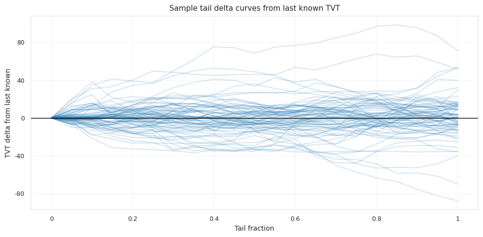
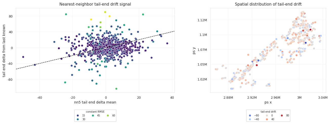
The last-known anchor is strong, but not sufficient. Some wells barely move in TVT, while others drift tens of feet or more. The model has to decide when to hold the anchor and when to follow a changing stratigraphic layer.

The constant-tail baseline is strong under common horizontal-well geometry. In many horizontal wells, the drilling objective is to stay within a target zone. If the well remains in zone, TVT can be nearly flat even while MD and X/Y change substantially. The same operational objective also creates the failure mode: when the well climbs, drops, crosses a boundary, or follows a dipping surface, the true TVT path may drift smoothly for thousands of rows. The estimator must preserve flat wells and still move on drifting wells.

The hidden tail is long enough that small bias compounds:

5 feet of persistent bias over 5,000 rows
is not a local error.
It is the whole tail placed in the wrong stratigraphic band.

The long-tail geometry turns the target into path modeling rather than isolated row prediction. Smoothing, slope clipping, and fade-in are part of the target geometry rather than cosmetic cleanup.

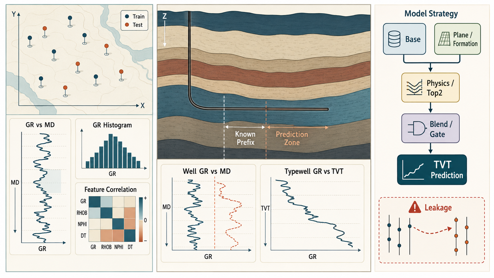
2. Leakage Boundary

The information boundary has two levels.

Mode	Allowed Evidence	Forbidden Evidence
Strict drilling-time	Prefix TVT_input, current row geometry, trailing windows, prefix-calibrated GR signals	Future rows, centered windows, tail length, tail TVT
Offline batch	Full provided test covariates such as future MD/X/Y/Z/GR, candidate paths, tail geometry	Tail TVT, target-derived summaries, direct train-only formation tops on test

The offline mode is not automatically leakage. Kaggle provides the full test covariate file, so future GR and geometry rows can be used as target-free signals. The key rule is narrower:

Future covariates are allowed only if they are available in the test file
and are not transformed through hidden target values.

This distinction separates two leakage cases.

Rejecting all full-tail features is too strict for the batch setting. The test file already contains the full well trajectory and the full GR sequence. A DTW path that uses the full horizontal GR trace is still target-free if it only aligns observed GR against the typewell GR curve. It is not simulating live drilling, but it is a valid batch estimator.

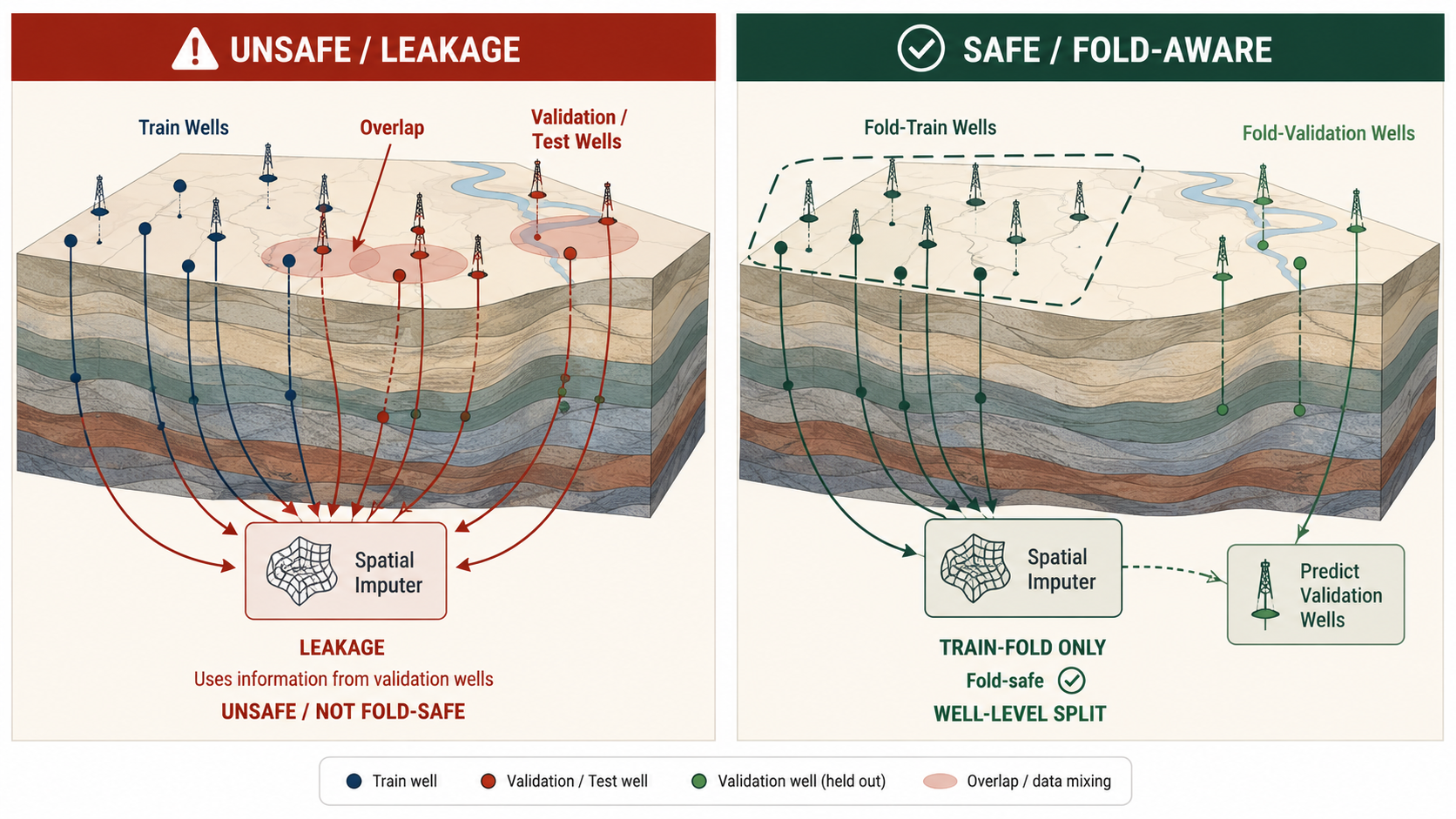
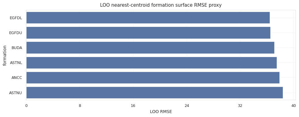
Treating every train-only geological column as safe is too loose. Formation tops such as ANCC, ASTNU, ASTNL, EGFDU, EGFDL, and BUDA are excellent explanatory variables in train, but they are not directly present in the test horizontal file. If a validation fold uses those true formation values from the held-out wells, the model is learning from a source that will not exist at inference. The safe version is a fold-trained imputer:

for train_idx, valid_idx in GroupKFold(n_splits=5).split(wells, groups=well_id):
    train_wells = wells.iloc[train_idx]
    valid_wells = wells.iloc[valid_idx]

    surface = fit_formation_surface(train_wells)
    valid_features = build_features(
        valid_wells,
        formation_source=surface,
        target_columns=None,
    )

The validation object must mimic the final inference object:

fit on training-fold wells
build target-free features for held-out wells
predict held-out hidden tails
score only hidden-tail TVT

Any shortcut that gives validation wells their own true tail labels, true formation tops, or target-derived summaries turns the fold into a memorization test.

The high-risk cases are:

Pattern	Risk	Safe Treatment
Row random split	Same-well autocorrelation leaks into validation	Use GroupKFold by well_id.
Formation tops in horizontal train file	Direct geological target proxy not present in test	Reconstruct only via fold-safe spatial imputation.
TVT_input backfill	Tail target copied backward	Use prefix only.
Tail TVT summaries	Direct target leakage	Exclude completely.
Nearby validation well labels	Spatial leakage across fold	Fit spatial/formation estimators on training-fold wells only.
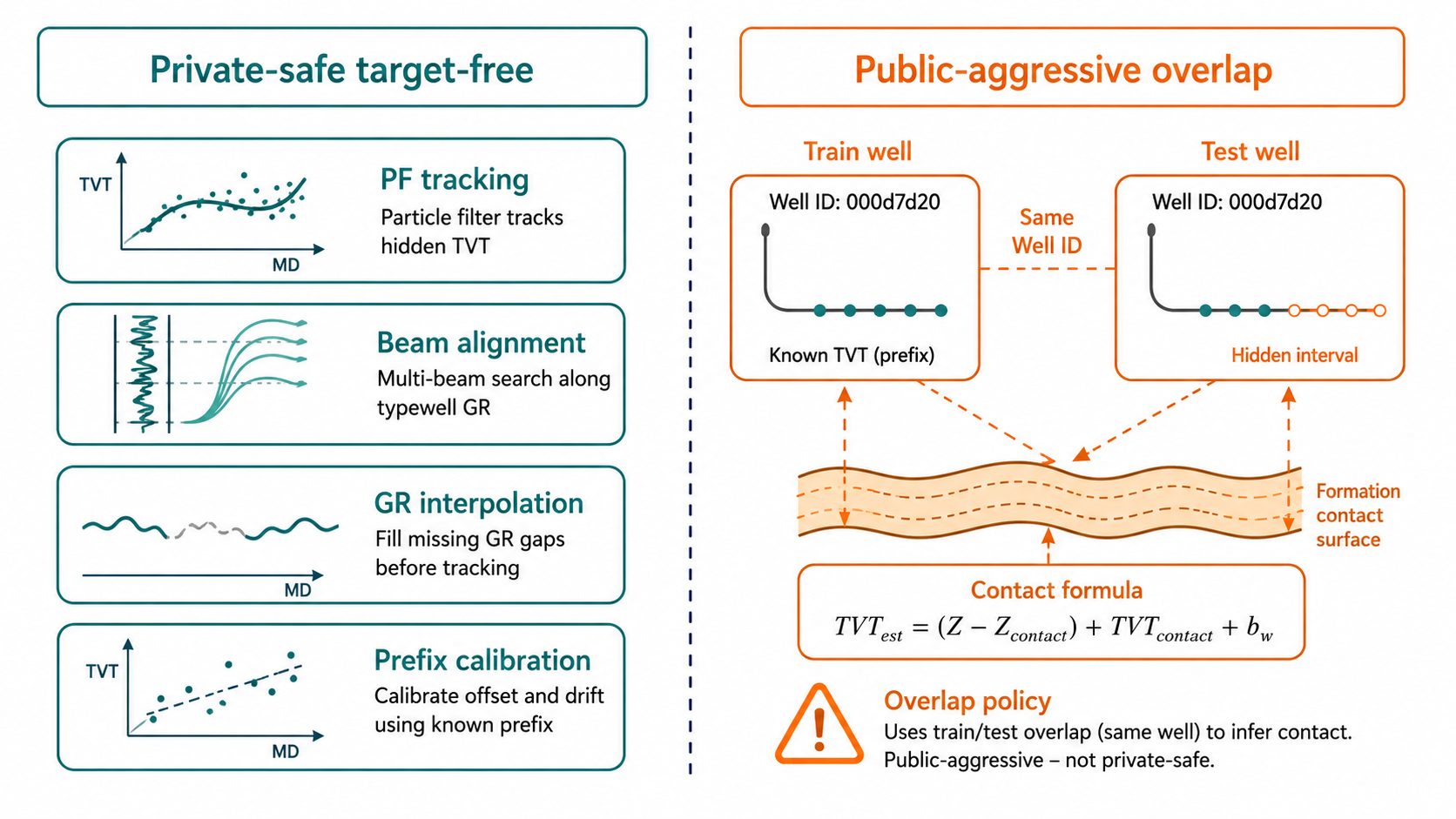
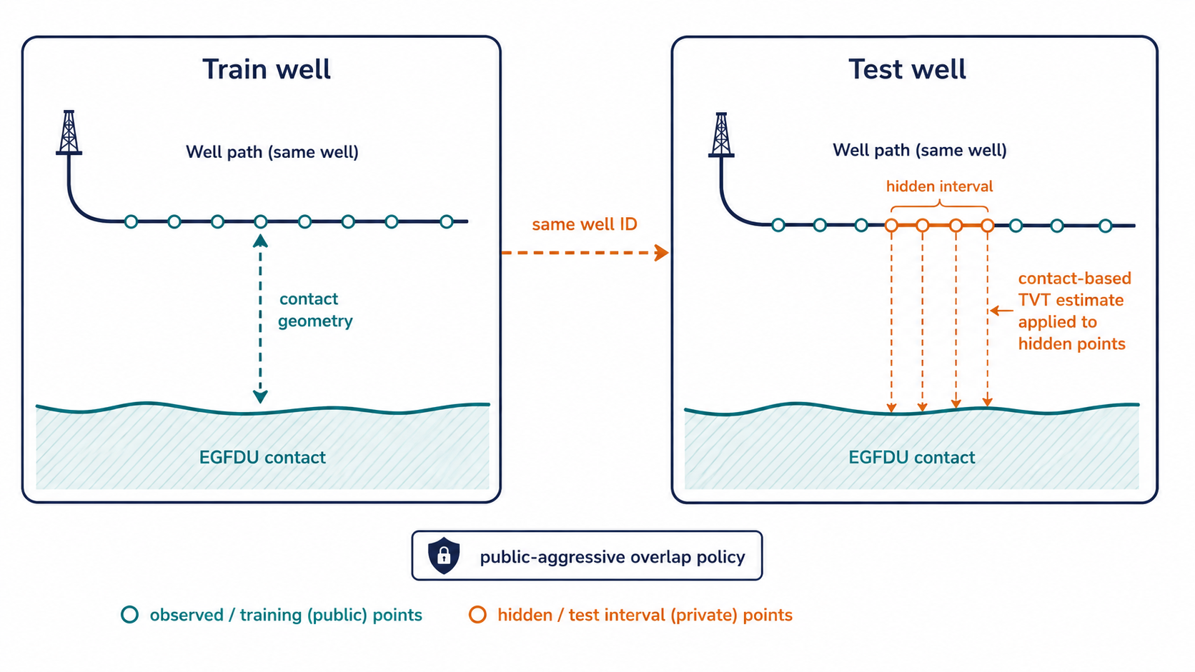
Same-well train/test overlap	Can dominate public LB if public wells repeat train IDs	Treat as public-aggressive, and compare with disabled mode.

The same-well physical path is not label leakage if it uses observable contact geometry and prefix-safe information. However, it is a public/private robustness risk. If public test wells overlap known train wells but private wells do not, the public score can reward a shortcut that does not generalize.

There are therefore two separate questions:

Question	Diagnostic
Is the estimator legal under the test-file information boundary?	Does it use only observable test covariates and prefix-safe information?
Is the estimator robust to a private split shift?	Does it still work when same-well overlap is disabled?

The public-aggressive branch can be legal but brittle. The private-safe branch can be less specialized but more informative about unseen wells. Separate reporting preserves interpretation. Mixing them into one unnamed score makes the evidence ambiguous.

The switch is explicit:

SUBMISSION_PROFILE = "pf_residual_gbdt"

# Public-aggressive overlap policy:
PF_SELECTOR_USE_SAME_WELL_PHYSICAL = True

# Private-safe robustness probe:
PF_SELECTOR_USE_SAME_WELL_PHYSICAL = False

The selector logic is:

\[\hat{T}^{selector}_i = \begin{cases} \hat{T}^{same\ well}_i, & \text{if same-well mode is enabled and a matching well is available} \\ \operatorname{Select}(H^{PF}, H^{beam}, H^{hold}\mid X,Y,Z,GR,T_{prefix}), & \text{otherwise} \end{cases}\]

Same-well contact sits outside the ordinary PF/beam selector. Same-well contact information behaves like a geometric shortcut. PF and beam behave like general stratigraphic trackers. An explicit switch keeps the public score auditable:

same-well on:
    public-overlap hypothesis

same-well off:
    unseen-well stratigraphic hypothesis

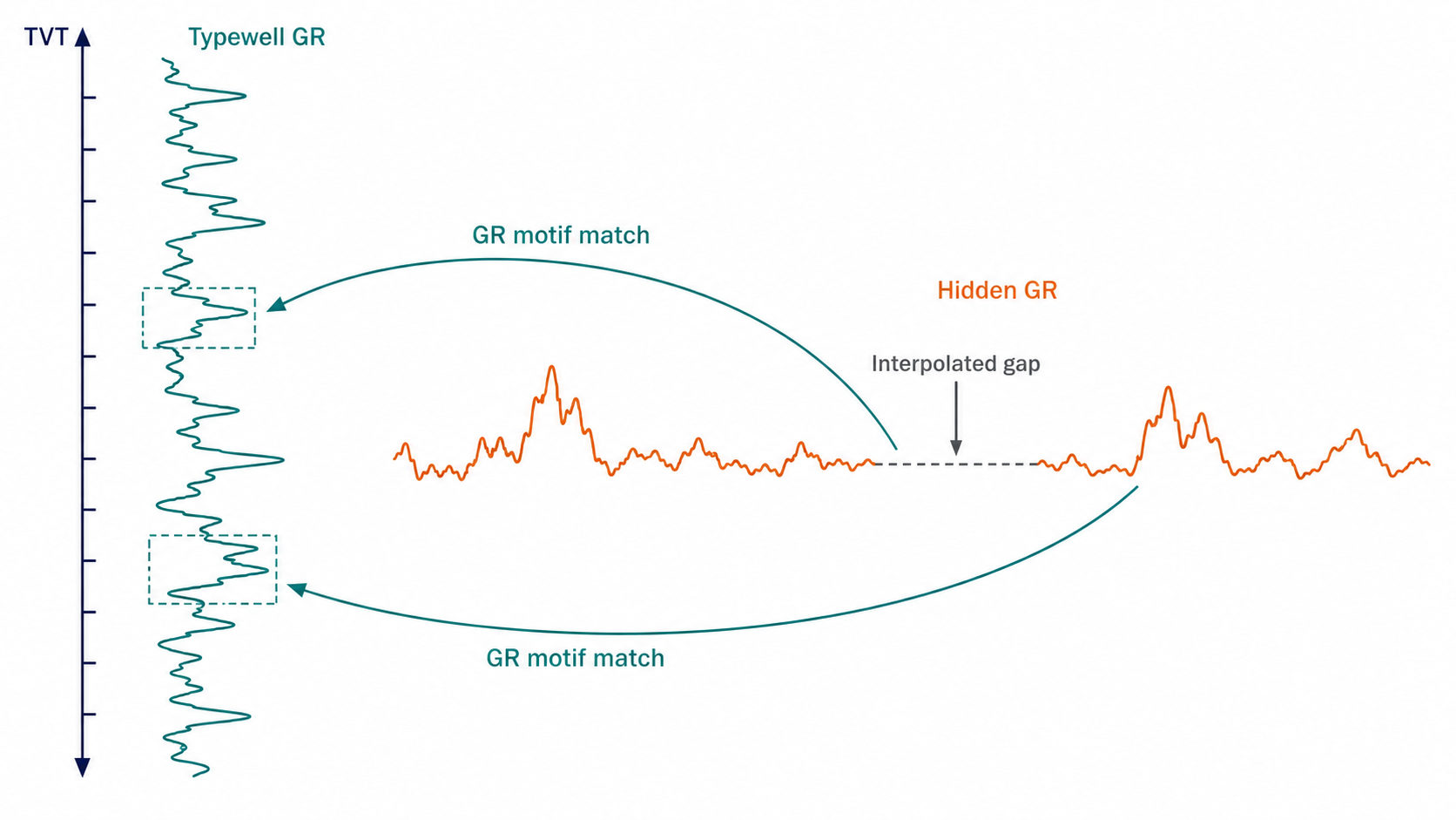
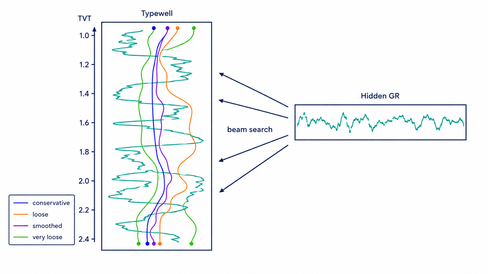
3. GR As A Stratigraphic Barcode

Gamma ray is not just another numeric feature. It is the main observable trace that links the horizontal well to the vertical typewell.
Gamma logs measure natural radioactivity around the borehole. In many sedimentary settings, shale-rich intervals and cleaner sand or carbonate intervals have different gamma responses, so the curve becomes a repeatable stratigraphic pattern. The absolute amplitude can vary by tool, borehole condition, and local geology, but the shape of the curve often carries layer-order information.

The typewell gives a reference curve:

TVT -> GR

The horizontal well gives a measured sequence:

MD -> GR

The problem is to infer the hidden mapping:

MD -> TVT

by aligning the horizontal GR sequence to the typewell GR sequence.

The alignment is not a simple lookup. A horizontal well can remain in one stratigraphic layer, cross a layer slowly, or encounter a local dip/fault/thickness change. The horizontal GR curve may therefore be a stretched, squeezed, shifted, or partially missing version of a typewell interval.

Several alignment families cover different deformation patterns:

Alignment Family	Handles Well	Fails When
Direct prefix calibration	Small local offset near prediction start	Tail drifts far from prefix behavior
DTW	Global stretching and squeezing of GR patterns	Missing GR gaps or repeated motifs create ambiguous matches
Beam path	Multiple local path hypotheses with constraints	Search grid misses the true path
PF	Sequential uncertainty and smooth motion	Likelihood is weak or noisy for long intervals
Formation estimate	Spatially coherent dipping surfaces	Local well-specific offset dominates

The GR curve does not uniquely determine TVT. It narrows the plausible set of TVT paths. The rest of the system decides which path is consistent with geometry, prefix calibration, formation position, and smoothness.

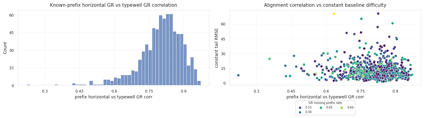
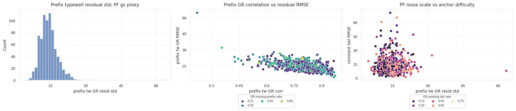
Prefix rows make this calibration measurable. For a prefix row with known TVT_input, compare horizontal GR to typewell GR at the same TVT:

\[r_i = GR^{horizontal}_i - GR^{typewell}(T^{input}_i)\]

The prefix residual scale:

\[\sigma_{GR,w} = \operatorname{std}(r_i)\]

becomes a well-specific observation-noise estimate. If the prefix correlation is weak or the residual scale is large, typewell matching should be trusted less.

Prefix calibration also protects against amplitude mismatch. Two wells can pass through similar stratigraphy but report GR on slightly different scales or baselines. A prefix-only affine adjustment:

\[GR^{calibrated}_i = a_w GR_i + c_w\]

can be fit on known prefix rows, then applied to the hidden tail without reading hidden TVT. The calibration is legal because it learns from the known prefix relation between horizontal GR and typewell GR. Leakage appears only if the tail TVT labels tune a_w or c_w.

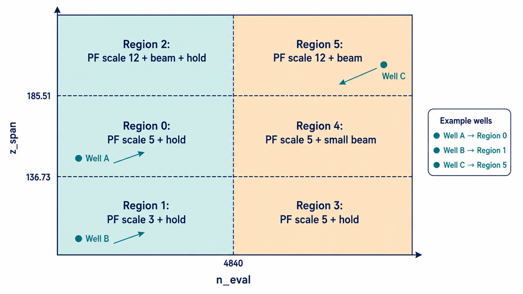
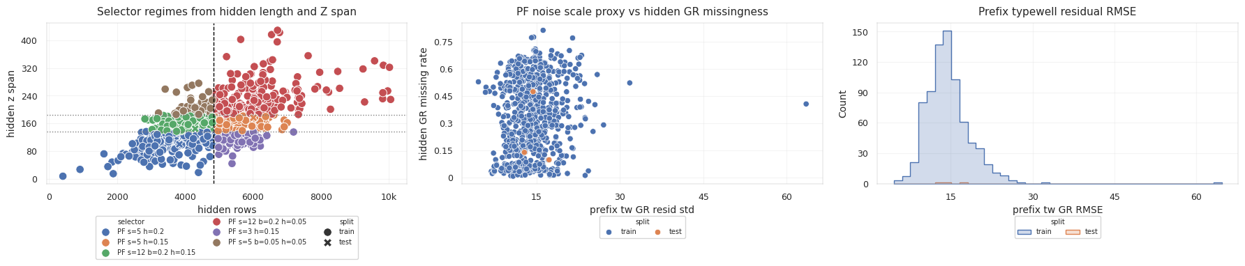
The test wells show three different reliability regimes:

Test Well	Hidden Rows	Hidden Z Span	Hidden GR Missing Rate	Prefix Typewell GR Corr	Selector Variant
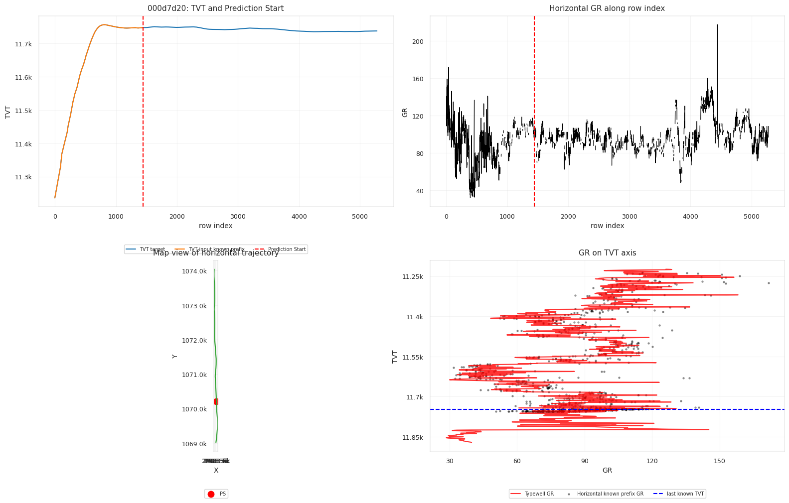
000d7d20	3836	100.02	0.4734	0.7718	pf_scale_5_hold_0.2
00bbac68	6014	176.49	0.1383	0.8274	pf_scale_5_hold_0.15
00e12e8b	4301	144.81	0.0972	0.9335	pf_scale_12_beam_0.2_hold_0.15

The third well has the cleanest prefix typewell correlation, so stronger alignment is plausible. The first well has much heavier hidden GR missingness, so the path must lean more on hold and geometry.

The selector variants reflect that reliability judgment:

Selector Component	Interpretation
pf_scale_3 or pf_scale_5	Narrower particle likelihood, used when GR evidence is relatively trustworthy.
pf_scale_12	Wider likelihood, used when the GR/typewell match needs more tolerance.
beam_0.2	Let a beam-aligned path contribute, but not dominate.
hold_0.15 or hold_0.2	Keep a fraction of the last-known anchor when evidence is uncertain.

The mode names are compact, but the meaning is geological: how much uncertainty to assign to the GR observation model, how much beam alignment to trust, and how much anchor inertia to preserve.

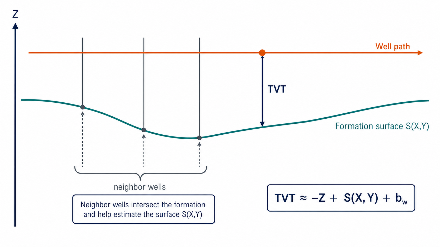
4. Formation Coordinates

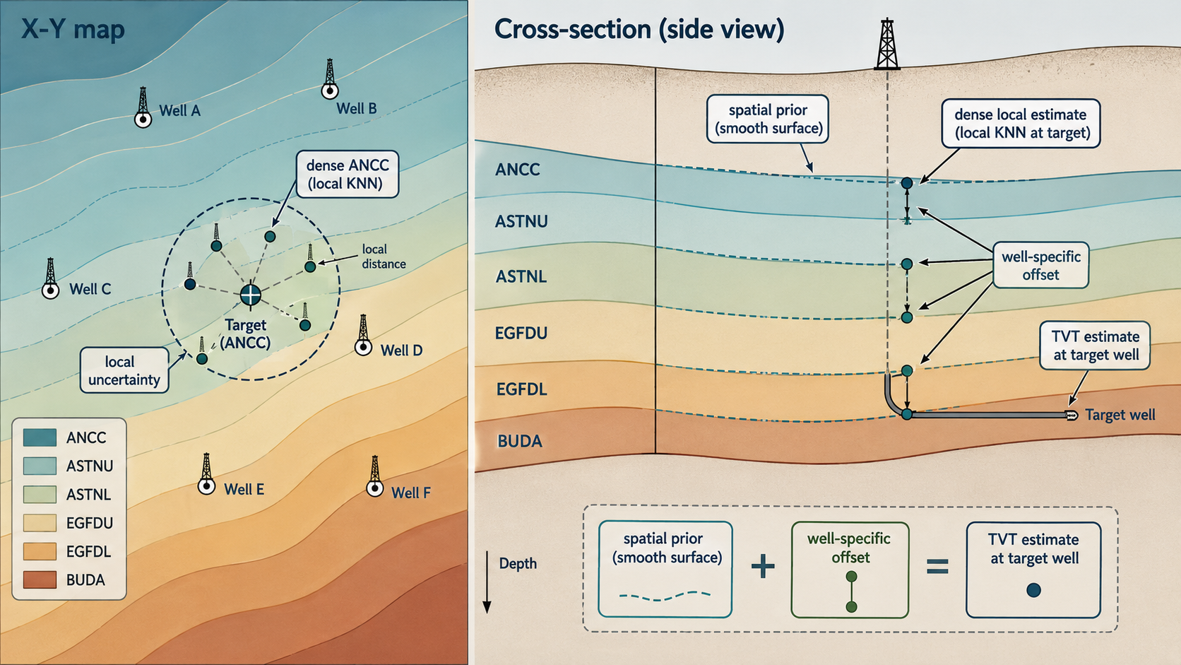
The geological relation behind the feature design is:

\[TVT_i \approx -Z_i + S(X_i,Y_i) + b_w\]

Equivalently:

\[TVT_i + Z_i \approx S(X_i,Y_i) + b_w\]

S(X,Y) is a structural surface, and b_w is a well-specific offset.
The relation makes TVT + Z often more stable than raw TVT: if the well moves through a dipping formation, Z changes because the borehole moves, while TVT + Z tracks the formation-relative coordinate.

One way to read the formula is:

observed vertical position:
    Z_i

estimated formation height at map location:
    S(X_i, Y_i)

well-specific local offset:
    b_w

stratigraphic coordinate:
    TVT_i

If the structure is nearly flat, S(X,Y) changes slowly and the anchor dominates. If the structure dips across the lateral path, S(X,Y) changes with location and a constant-TVT path becomes less plausible. If the well has a local landing offset, the prefix estimates b_w.

Spatial geology enters row-wise prediction through this relation. The inference question is not only, “What does row 3000 look like?” It is:

At this X/Y location and this Z depth,
where should the target stratigraphic coordinate be
relative to the formation surface and prefix offset?

The safe formation pattern is:

# fit only on training-fold wells
formation_model.fit(train_fold_xy, train_fold_formation_top)

# project validation or test rows from observable X/Y
formation_hat = formation_model.predict(row_xy)

# combine with row Z and prefix offset
tvt_estimate = -z + formation_hat + prefix_bias

The unsafe pattern is direct use of formation columns that exist in the train horizontal file but not in the test horizontal file. Those columns are excellent EDA evidence, but they must be converted into reproducible, fold-safe estimators before entering validation or inference.

The conversion has two roles.

First, it makes the feature available at test time. A model cannot rely on a column that will not exist in the final test horizontal file.

Second, it makes validation honest. If validation wells receive true formation tops while test wells receive imputed surfaces, validation measures a different problem. Fold-safe surface estimation forces the validation fold to live with the same approximation error that test inference will have.

The effective signal is not the raw formation top itself. The effective signal is the residual geometry after projecting an estimated surface:

\[\epsilon^{formation}_i = (TVT_i + Z_i) - \hat{S}(X_i,Y_i)\]

In the prefix, this residual estimates local offset. In the tail, the same estimated surface provides a target-free trajectory prior.

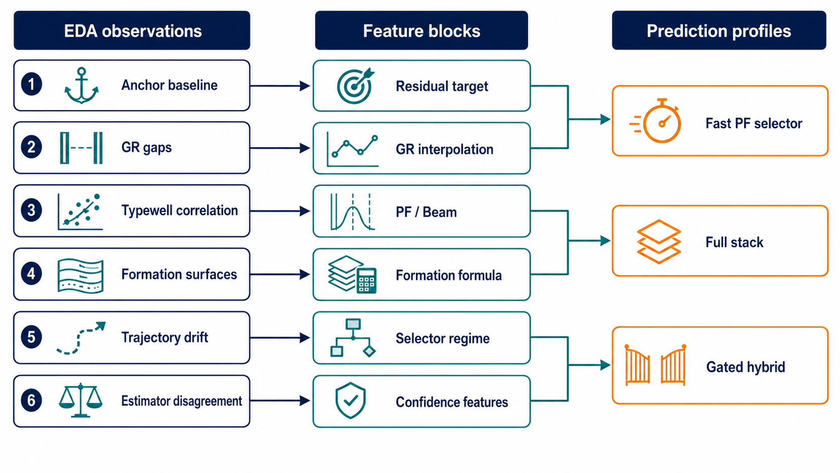
5. EDA Signals That Become Features

EDA enters the model only when each observation becomes a controlled feature family.
The mapping is:

Observation	Geological Meaning	Feature Family
Long single hidden tail	Prediction is a trajectory, not isolated rows	tail_frac, md_since_last_known, fade-in from anchor
Small per-row TVT steps	True path should be smooth	slope clipping, local smoothing, jump penalties
Large tail range in some wells	Anchor hold is not enough	PF, beam, DTW, formation drift
GR missing gaps	Observation likelihood is unreliable	missing-rate features, long-gap flags, fallback holds
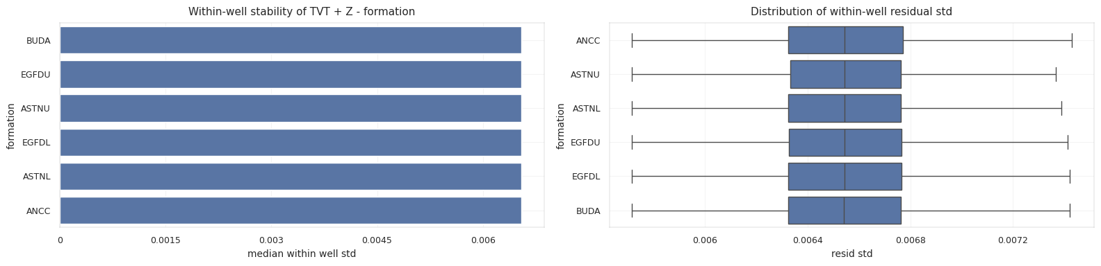
Prefix GR/typewell mismatch	Typewell alignment reliability varies by well	prefix correlation, RMSE, residual std
TVT + Z stability	Formation-relative coordinate exists	formation-plane and formation-top estimates
Same-well overlap	Strong public shortcut, private risk	separate public-aggressive and private-safe profiles

The middle column enforces the conversion from plot to feature. Raw plots do not become features directly. Each plot first becomes a geological statement, then that statement becomes a leak-safe feature. For example:

Plot:
    tail TVT is smooth with rare jumps

Geological statement:
    plausible hidden paths should have bounded slope

Feature or postprocess:
    train-derived slope quantile, fade-in, slope clipping

The same translation applies to GR gaps:

Plot:
    some hidden tails contain long GR NaN runs

Geological statement:
    observation likelihood is weaker inside gaps

Feature or postprocess:
    missing-rate flags, longest-gap features, hold weight, lower alignment confidence

This prevents the model from treating every diagnostic as a numeric invitation. If a diagnostic cannot be reproduced from legal test-time information, it stays in EDA.

The trajectory features come from measured geometry:

\[\frac{dZ}{dMD} = \frac{Z_i - Z_{i-1}}{MD_i - MD_{i-1}}\] \[dXY_i = \sqrt{(X_i-X_{i-1})^2 + (Y_i-Y_{i-1})^2}\]

Curvature is estimated from changes in normalized trajectory direction. These are not target features. They describe how the borehole moves through space, which constrains how fast TVT can plausibly move.

The geometry features are not expected to solve TVT alone. They provide priors:

Geometry Signal	Constraint On TVT
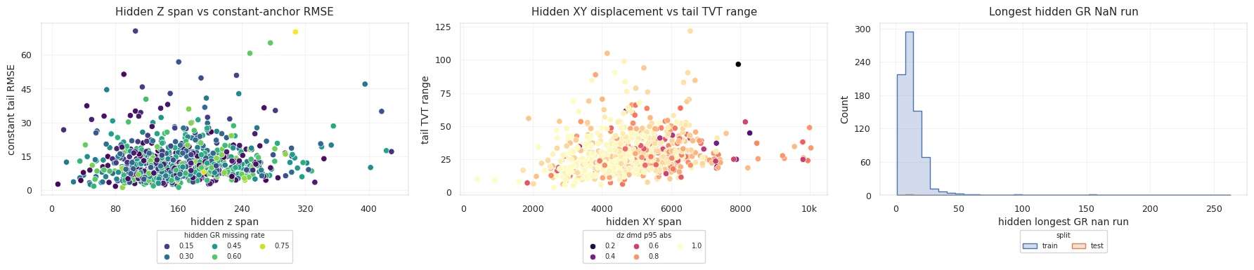
Small hidden_z_span	Less vertical movement, stronger anchor plausibility.
Large hidden_z_span	More room for formation crossing or drift.
Stable azimuth	Smoother structural trend along the lateral.
High curvature	Local steering changes can break a simple linear path.
Long MD tail	Small per-row bias can accumulate over many rows.

The residual model can then learn that the same GR disagreement has different meaning in a short flat tail and in a long dipping tail.

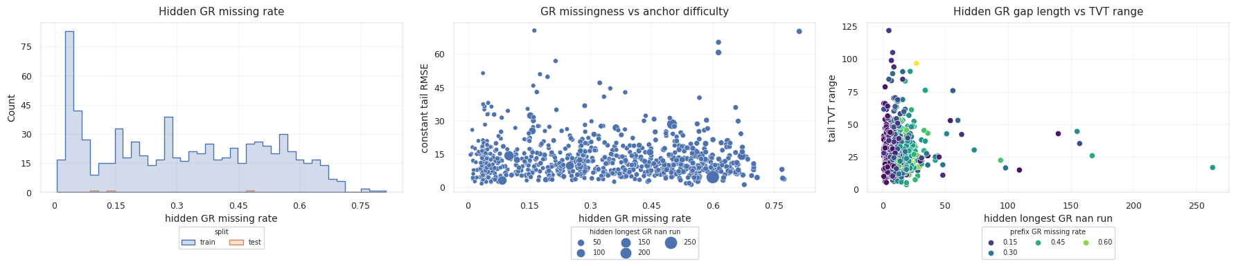
GR quality controls the observation model. A long missing interval should not be interpreted as evidence for a flat TVT path, nor as evidence for a sharp drift. It is simply lower information density.

For a PF or beam path, missing GR changes the likelihood surface. In observed intervals, GR can sharply favor one TVT band over another. In missing intervals, the estimator has to propagate the previous state through motion constraints. Missingness features and hold weights therefore become part of the path model:

observed GR:
    update path likelihood

missing GR:
    propagate path under smoothness and geometry priors

long missing GR:
    increase uncertainty and shrink corrections

The target itself is smooth but not trivial. The median absolute step is tiny, but rare jumps and long-tail drift make a naive constant path fragile.

The slope clip is derived from the training distribution, not chosen as an arbitrary visual smoother. If the 90th percentile of absolute TVT step is used, the postprocess encodes:

Most true paths do not move faster than this per-row rate.
Predictions may move, but must justify movement through many consistent rows.

That is a different operation from simply applying a rolling mean. It preserves long drift while suppressing isolated spikes that contradict the physical continuity of the well path.

Typewell inventory and prefix diagnostics determine how much trust to assign to barcode matching:

The constant-anchor baseline is the reference point. Many wells stay near the last known TVT, so a model must earn its drift. A complex alignment model that moves flat wells unnecessarily can score worse than the anchor.

This baseline also gives a clean error decomposition:

If Anchor Fails Because…	Needed Signal
TVT drifts with formation dip	X/Y/Z formation surface and trajectory slope
GR pattern shifts to another layer	typewell alignment, DTW, beam, PF
Prefix offset is misleading	nearby-well or formation residual correction
Long tail accumulates small drift	gradual residual model plus fade-in
GR is missing or ambiguous	hold path and uncertainty-aware gate

The metric is row-weighted, so long tails dominate. Well-level diagnostics are still necessary because a few very long wells can hide systematic failure on shorter wells.

\[RMSE_{row} = \sqrt{ \frac{1}{N} \sum_i (\hat{T}_i - T_i)^2 }\] \[RMSE_{well} = \frac{1}{W} \sum_w \sqrt{ \frac{1}{n_w} \sum_{i \in w} (\hat{T}_i - T_i)^2 }\]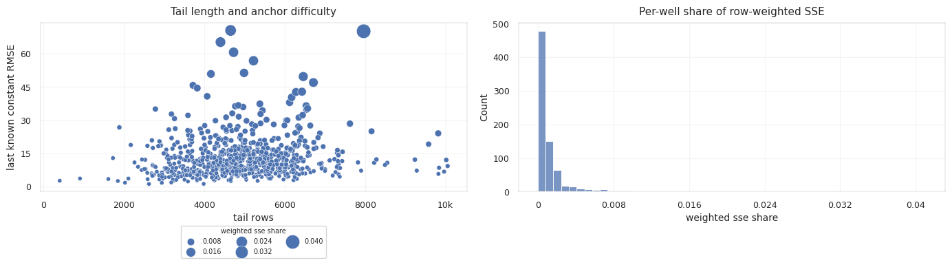

Curve-level diagnostics, dense surface estimates, nearby-well spatial signals, and representative well plots are used as reliability checks rather than as raw output dumps.

The final feature pipeline keeps the EDA interpretation attached to leakage policy:

6. Feature Policies

Feature sets are separated by policy:

Feature Set	Policy	Feature Count
causal_base	strict	39
prefix_context	strict	60
typewell_alignment	strict	108
calibrated_typewell_alignment	strict	137
offline_prefix_context	offline	115
offline_typewell_alignment	offline	163
offline_calibrated_typewell_alignment	offline	192
offline_candidate_path_alignment	offline	263
offline_candidate_path_calibrated_alignment	offline	292
offline_formation_plane_alignment	offline	223
offline_formation_top_alignment	offline	246
offline_beam_candidate_path_alignment	offline	298
offline_super220_alignment	offline	220
offline_compact_lgbm_style	offline	83
offline_compact_lgbm_formation_style	offline	143
offline_compact_lgbm_formation_top_style	offline	166

The selected strict feature set is calibrated_typewell_alignment, with:

Setting	Value
feature count	137
shrinkage alpha	0.81183
fade-in tau MD	200
slope clip	True
slope quantile	0.9

The best stored offline feature family is offline_candidate_path_alignment, with stronger shrinkage:

Setting	Value
feature count	263
shrinkage alpha	0.94115
fade-in tau MD	200
slope clip	True
slope quantile	0.9

The distinction is conceptual:

strict features test drilling-time robustness
offline features exploit full provided test covariates without touching hidden targets

7. Validation Philosophy

Validation has to answer a geological generalization question:

Can the estimator recover the hidden TVT tail of a well
whose tail labels were not visible during fitting?

A row random split answers a weaker question:

Can the estimator interpolate rows from a well
whose neighboring rows and same-well patterns were already visible?

That weaker question is too optimistic. Wells are strongly autocorrelated. Consecutive rows share trajectory, GR context, prefix behavior, and formation position. A row split can let a model learn a well-specific curve and then appear to predict held-out rows from the same curve.

The validation unit is therefore the well:

groups = train_tail["well_id"]

for fit_idx, valid_idx in GroupKFold(n_splits=5).split(train_tail, groups=groups):
    fit_rows = train_tail.iloc[fit_idx]
    valid_rows = train_tail.iloc[valid_idx]

    fit_package = fit_all_estimators(fit_rows)
    valid_pred = infer_hidden_tail(valid_rows, fit_package)
    fold_rmse = rmse(valid_rows["TVT"], valid_pred)

The fold package has to contain the same categories of objects that final inference will use:

Object	Fold Behavior	Final Behavior
Typewell calibration	Fit prefix relations for held-out validation wells only from their known prefix	Fit prefix relations for test wells only from their known prefix
Formation surface	Fit from training-fold wells	Fit from all allowed training wells
PF/beam/DTW paths	Build from held-out covariates and typewell curves	Build from test covariates and typewell curves
Residual model	Train on fit-fold residuals	Train on all training residuals
Postprocess policy	Select globally, then apply to held-out predictions	Apply the selected policy to test predictions

The public/private distinction sits on top of this validation design. A feature can pass GroupKFold and still be public-fragile if it depends on same-well overlap. A feature can be offline-safe and still private-robust if it uses full test GR/trajectory covariates without relying on overlap. Separate reporting keeps those categories from collapsing into one score.

Three scores answer three different questions:

Evidence	Question Answered
Strict GroupKFold	Can the model work with prefix/current/trailing information only?
Offline target-free GroupKFold	How much does the full covariate path help without hidden target leakage?
Public same-well enabled submission	How much does observed public overlap improve the visible leaderboard?

The final choice depends on risk tolerance. A high public score can be rational if the overlap signal is expected to remain present. A private-safe submission should still have a strong target-free core when overlap is removed.

8. PF, Beam, DTW, And Selector Modes

The estimator family is not a single path. It is a set of candidate trajectories:

Candidate	Meaning
hold	Stay near last known TVT_input.
PF	Particle-filter path through possible TVT states, weighted by GR/typewell likelihood and motion constraints.
beam	Deterministic beam search over plausible TVT paths.
DTW	Global sequence alignment between horizontal GR and typewell GR.
formation path	Convert X/Y/Z through a safe formation surface estimate.
same-well physical	Contact/geometry estimate for overlapping train/test well IDs.

Each candidate encodes a different failure assumption.

The hold path assumes the well remains in the same stratigraphic position. It is hard to beat on flat tails and dangerous on drifting tails.
The formation path assumes spatial structure dominates. It can follow dipping geology even when GR is missing, but it can miss local well-specific offsets.
The GR alignment paths assume the typewell barcode is informative. They can detect stratigraphic movement, but repeated GR motifs can create false matches.
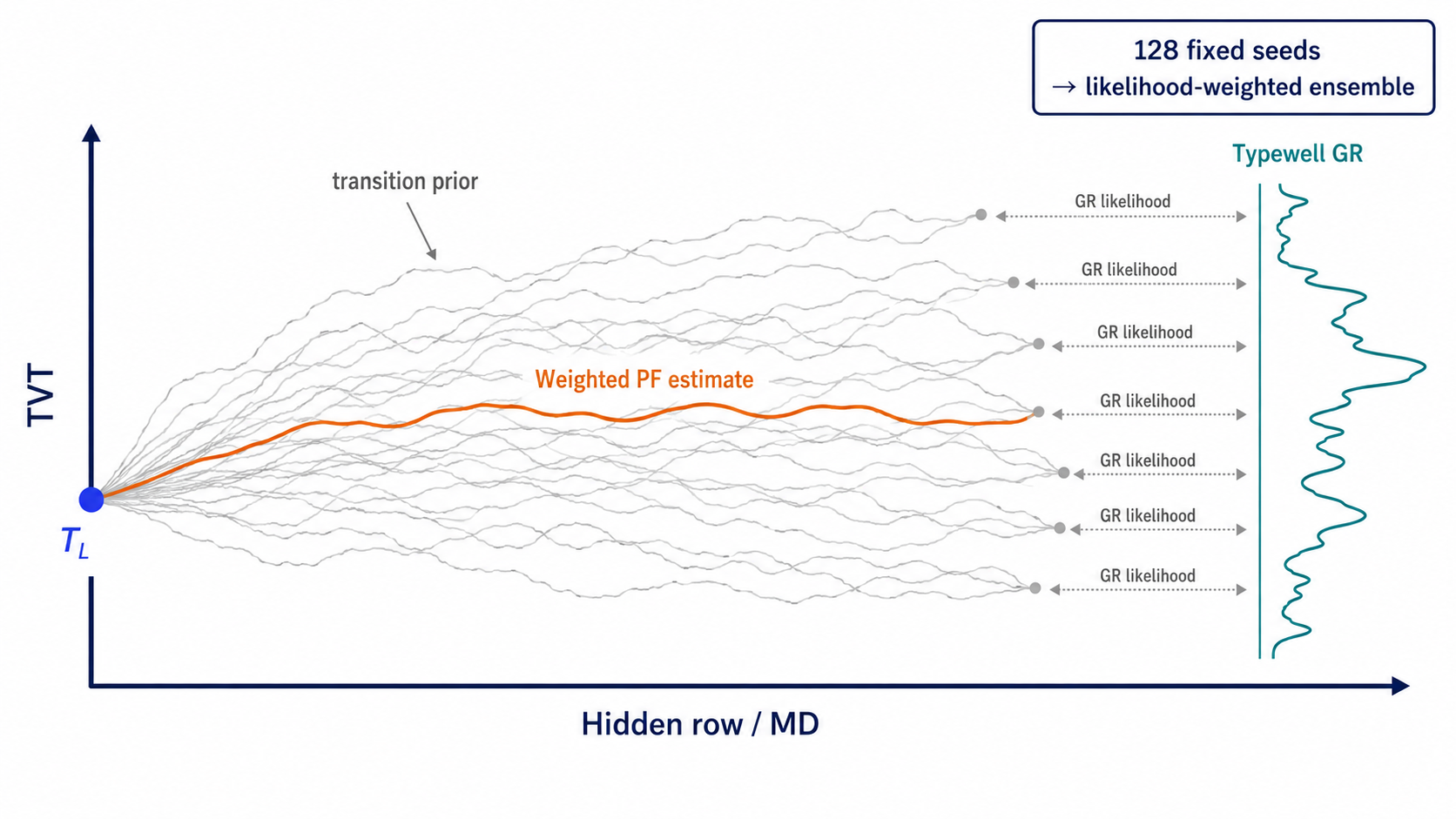
The PF path assumes uncertainty should be carried forward sequentially rather than collapsed into one best alignment too early.

The particle-filter state can be read as:

\[s_i = TVT_i\]

with a transition prior:

\[p(s_i \mid s_{i-1}) \propto \exp \left( - \frac{(s_i - s_{i-1} - \mu_i)^2}{2\tau_i^2} \right)\]

and an observation likelihood:

\[p(GR_i \mid s_i) \propto \exp \left( - \frac{(GR_i - GR^{typewell}(s_i))^2}{2\sigma_{GR,w}^2} \right)\]

Here mu_i can reflect expected drift from geometry or previous path behavior, while sigma_GR,w is prefix-calibrated. Missing GR rows flatten the observation likelihood, so the transition prior and hold/formation components matter more.

The beam path is less probabilistic. It keeps a limited set of plausible partial paths and extends them under local costs. This prevents a single greedy path from locking onto an early false match. Beam search can keep several nearby stratigraphic hypotheses alive until later GR evidence separates them.

The DTW recurrence is:

\[D(i,j) = (GR^{h}_i - GR^{tw}_j)^2 + \min \left[ D(i-1,j-1), D(i-1,j), D(i,j-1) \right]\]

It is target-free because it aligns GR sequences, not TVT labels. Its danger is not label leakage; its danger is overtrusting noisy or missing GR.

DTW permits local stretching:

horizontal segment A may correspond to a short typewell interval
horizontal segment B may correspond to a longer typewell interval

That flexibility matches real stratigraphic correlation, where layers can thicken, thin, or be drilled at different angles. The same flexibility can also overfit noise. A repeated GR motif may let DTW choose a visually plausible but geologically shifted band. DTW therefore remains one candidate signal rather than a standalone oracle.

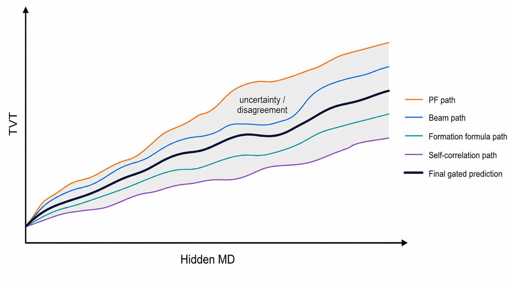
When estimators disagree, the disagreement itself becomes an uncertainty signal. A high-confidence correction is small when PF, beam, formation, and hold paths cluster together. A large divergence means the final blend should shrink toward safer paths.

The disagreement features are often more valuable than the raw path values:

Disagreement	Interpretation
PF close to beam, far from hold	GR evidence consistently supports drift.
PF close to hold, beam far away	Beam may be following a false GR match.
Formation close to hold, GR paths far away	GR motif may be ambiguous or locally miscalibrated.
All paths spread out	High uncertainty, prefer shrinkage and small corrections.
Same-well physical far from target-free paths	Public-overlap shortcut conflicts with general geology.

This converts model conflict into a first-class feature rather than hiding it inside a blind ensemble.

The selector regime map summarizes which mode is plausible by well context:

The registry audit keeps feature families and policies visible:

9. Submission Profiles

Profiles encode different risk positions:

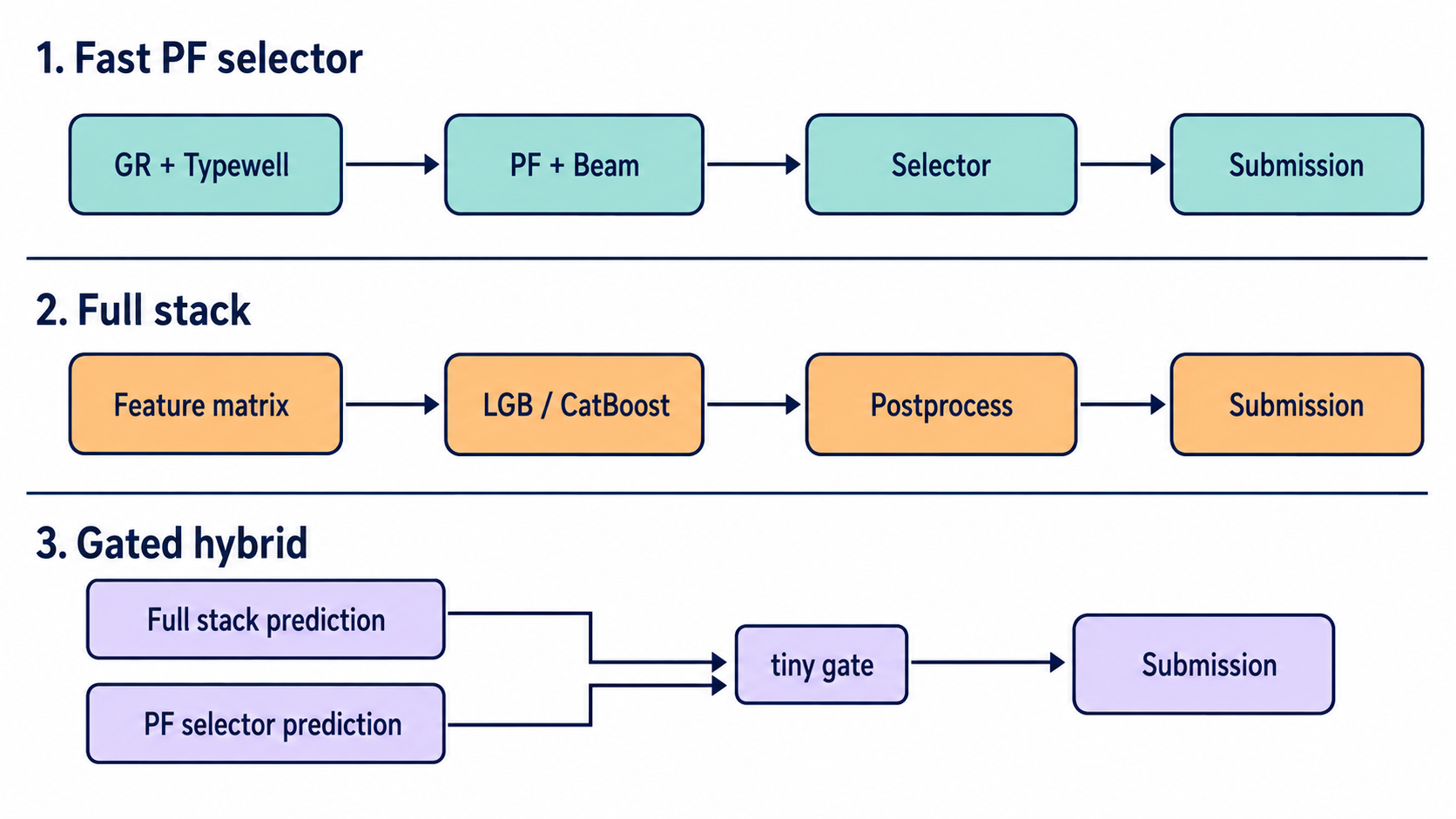
Profile	Interpretation
fast_pf_selector	Target-free PF/beam selector. Useful for selector reproduction and quick probing.
fast_pf_selector_128	Same family with more PF seeds. Lower Monte Carlo noise, higher runtime.
model_package_only	Run the packaged model inference without the PF/stack base.
pf_residual_gbdt_exact	Public PF-residual GBDT reproduction mode with exact-style feature handling.
pf_residual_gbdt	Guarded PF-residual GBDT variant with median-guarded fills.
full_stack_postproc	Full target-free stack plus post-processing.
full_stack_sel15_gated	Full stack with a small gated PF selector correction.
full_stack_postproc_model_gated	Post-processed stack plus gated model-package correction.
full_stack_postproc_model_late	Post-processed stack plus fixed-weight model-package correction.
full_stack_sel15_gated_model_gated	Selector blend plus gated model-package correction.
full_stack_sel15_gated_model_late	Selector blend plus late fixed-weight model correction.

The profiles fall into four families:

Family	Profiles	Main Question
PF selector	fast_pf_selector, fast_pf_selector_128	How strong is the target-free path selector without residual modeling?
Model package	model_package_only	Can the learned package reproduce test inference by itself?
PF residual	pf_residual_gbdt_exact, pf_residual_gbdt	How much systematic PF bias can GBDT remove?
Full stack plus correction	full_stack_*	How much can multiple target-free estimators and sidecar corrections safely move the base?

The profile name determines more than runtime. It determines which evidence source is allowed to control the final prediction:

selector profile:
    path choice dominates

residual profile:
    PF path dominates, GBDT corrects bias

full stack profile:
    many target-free hypotheses compete through stack weights

model-gated profile:
    external model-package inference can move the base only through a gate

The gated stack/selector correction uses disagreement-sensitive shrinkage:

\[g_i = \frac{g_{max}} {1 + \left(\frac{|\hat{T}^{selector}_i - \hat{T}^{stack}_i|}{s}\right)^2}\] \[\hat{T}^{final}_i = (1-g_i)\hat{T}^{stack}_i + g_i\hat{T}^{selector}_i\]

The same gate form applies to model-package sidecar blends:

\[\operatorname{GateBlend}_i(A,B) = (1-G_i)A_i + G_iB_i\]

A fixed late blend is simpler:

\[\hat{T}^{final}_i = (1-w)A_i + wB_i\]

The gate protects against estimator-specific failure. Two strong target-free estimators can fail on different wells. A blind average can move correct rows away from the geological path. A disagreement-aware gate makes the correction small exactly where model conflict is high.

10. PF-Residual GBDT

The guarded PF-residual profile starts with a PF path and trains tree models on the residual:

\[R_i = T_i - \hat{T}^{PF}_i\]

The final form is:

\[\hat{T}^{final}_i = \hat{T}^{PF}_i + 0.40 f_{lgb}(x_i) + 0.40 f_{xgb}(x_i) + 0.20 f_{cat}(x_i)\]

The tree models do not replace the physical path. They learn systematic PF bias:

Component	Function
PF base	Provides a target-free geological trajectory.
Residual features	Describe reliability, geometry, prefix calibration, and path disagreement.
GBDT correction	Adjusts predictable PF bias under GroupKFold validation.
Guarded fills	Prevents missing or unstable features from producing extreme corrections.

The residual framing acts as a regularization device. Direct TVT prediction can learn broad well-level levels and row-position effects that look strong in local validation but are hard to interpret geologically. PF-residual prediction forces the learned correction to answer a narrower question:

Given a physically plausible PF path,
when is that path systematically too high or too low?

Examples:

Residual Pattern	Possible Explanation
PF too flat after long Z drift	Formation dip is underweighted.
PF overreacts inside GR gaps	Missing GR interpolation is too confident.
PF shifted by a nearly constant offset	Prefix GR/typewell calibration or formation offset is biased.
PF follows a false motif	Beam/DTW disagreement and prefix correlation should reduce trust.

The residual model can correct those cases without being allowed to invent a completely unconstrained path. The final postprocess then limits the correction with shrinkage, fade-in, and slope clipping.

The OOF result:

Fold	Residual RMSE	Absolute TVT RMSE
1	9.6520	9.6520
2	10.2444	10.2444
3	9.7082	9.7082
4	10.5604	10.5604
5	12.4396	12.4396

Model	OOF Absolute RMSE
PF only	11.0106
PF + residual GBDT	10.5696

The correction is small enough to preserve the physical prior, but large enough to absorb repeatable PF errors.

The fold spread identifies heterogeneous failure modes. Fold 5 is worse than the other folds, which means some held-out well group is harder under the same estimator. Average RMSE alone does not identify whether the worst fold is caused by a specific failure mode:

high GR missingness
weak prefix correlation
large hidden Z span
unusual formation offset
same-well branch unavailable

Those diagnostics determine whether the next improvement should be a stronger model, a safer gate, a better formation surface, or a more conservative hold policy.

The core idea is visible in the feature policy table:

feature_policies = {
    "anchor_residual": "strict",
    "gr_quality": "target_free",
    "prefix_typewell_calibration": "strict",
    "pf_state_space": "target_free",
    "beam_alignment": "target_free",
    "selector_regime": "target_free",
    "same_well_physical": "public_aggressive",
}

Leakage control lives in the feature policy labels. Each feature family carries a policy label, so a strong score is interpretable as a combination of strict, target-free offline, and public-aggressive evidence rather than a single undifferentiated feature matrix.

11. OOF Artifacts And Model-Package Inference

OOF predictions are validation evidence. They are not a complete submission engine.

An OOF artifact answers:

How did the estimator behave on held-out training wells?

The final submission needs:

What is the estimator's prediction for the hidden rows in the test wells?

Those are different objects. The hidden test rows do not have OOF predictions because they were never validation targets. Therefore a reusable package must contain enough machinery to recreate inference:

Many strong signals are generated by procedures, not by static columns. A PF path is produced by running a state tracker on the test well. A beam path is produced by searching against the typewell curve. A formation feature is produced by fitting and applying a spatial estimator. A model package that only ships OOF numbers has none of that machinery for the test rows.

The reusable artifact therefore needs two layers:

Layer	Contents
Evidence artifact	OOF predictions, fold scores, feature importance, validation diagnostics
Inference artifact	feature builder, fitted imputers, fitted models, profile config, postprocess config

The evidence layer measures validation behavior. The inference layer produces submission.csv.

Required Piece	Reason
Feature builder	Test rows need the same target-free geometry, GR, PF, beam, and formation features.
Prefix calibration	Test wells need their own prefix GR/typewell reliability estimates.
Safe imputers	Formation and spatial estimates must be reproducible without validation labels.
Trained models	Residual correction needs final fitted LGB/XGB/CatBoost or stack components.
Sample alignment	Sidecar output must match sample_submission.csv row order exactly.
Blend policy	Base and sidecar predictions need a fixed off, late_linear, or gated_late_linear rule.

A compact package manifest acts as a reproducibility contract:

package/
    config.json
    feature_registry.json
    formation_surface.pkl
    typewell_calibration.py
    pf_config.json
    beam_config.json
    lgb_models/
    xgb_models/
    catboost_models/
    postprocess.json

The contract determines the package content:

Given only competition train/test files and the package,
the package can rebuild the same test feature matrix
and produce the same id-ordered predictions.

The inference contract is:

sample = pd.read_csv("sample_submission.csv")
base = build_target_free_base_submission(test_files, sample)

sidecar = run_model_package_inference(
    test_horizontal_files,
    test_typewell_files,
    sample_submission=sample,
)

base = align_submission_to_sample(base, sample)
sidecar = align_submission_to_sample(sidecar, sample)

final = blend_base_and_sidecar(base, sidecar, mode=SIDECAR_MODE)

The sidecar separates the high-confidence base from optional learned corrections. The base can be a PF-residual or full-stack target-free submission. The sidecar can be a model package trained from a different feature family. The final blend then asks whether the sidecar should move the base, not whether the sidecar should replace it.

The alignment guard is non-negotiable:

def align_submission_to_sample(frame, sample, label):
    frame = frame[["id", "tvt"]].copy()
    frame["id"] = frame["id"].astype(str)
    aligned = sample[["id"]].merge(frame, on="id", how="left")

    if aligned["tvt"].isna().any():
        raise ValueError(f"{label}: missing predictions after id alignment")

    return aligned

The sidecar correction is deliberately optional:

Sidecar Mode	Behavior
off	Keep the base submission unchanged.
late_linear	Apply a fixed late weight to the sidecar estimate.
gated_late_linear	Apply a small correction only where base/sidecar disagreement is within the gate scale.

With SIDECAR_MODE = off, the final file remains the guarded PF-residual GBDT submission. The sidecar path still defines a safe way to consume model-package predictions when they are available: model inference runs on test covariates, aligns by sample IDs, and moves the base only through a fixed contract.

The gated sidecar correction follows the same uncertainty logic as the PF/beam stack. If the base and sidecar agree, the correction is low-risk because two independent routes found the same stratigraphic band. If they disagree sharply, the gate reduces the movement:

\[G_i = \frac{G_{max}} {1 + \left(\frac{|B_i - A_i|}{s}\right)^2}\] \[\hat{T}_i = (1-G_i)A_i + G_iB_i\]

where A_i is the selected base, B_i is the sidecar prediction, G_max is a hard movement budget, and s is the disagreement scale.

The sidecar diagnostics should report:

Diagnostic	Meaning
aligned row count	Whether the sidecar covers every sample row.
missing IDs	Whether the package failed to infer any submission row.
mean absolute difference	Typical sidecar movement from base.
p95 absolute difference	Tail risk of the correction.
effective gate mean	Average sidecar weight after gating.
max correction	Worst-case movement allowed by the final blend.

Without those diagnostics, a sidecar blend can silently become a second submission hidden inside the first. With them, it remains a controlled correction.

12. Super Stack Logic

The larger stack combines several target-free pseudo-TVT paths:

Signal	Role
Beam	Discrete stratigraphic path search over typewell GR.
DTW	Global sequence alignment between horizontal and typewell GR.
Self-correlation	Internal GR pattern consistency along the well.
Formation planes	Structural X/Y/Z priors.
Dense ANCC proxy	Safe spatial proxy for formation geometry.
PF	Sequential state tracking with likelihood and motion constraints.
Trajectory	Borehole geometry and smoothness priors.

The stack uses nonlinear reliability models, positive linear blending, sparse hill-climb search, and post-processing:

candidate paths
-> shared target-free feature matrix
-> LGB / CatBoost residual models
-> ridge or sparse blend
-> shrinkage toward anchor
-> fade-in from prefix
-> slope clipping and smoothing
-> submission contract guard

The stack covers different estimator biases:

Estimator	Typical Bias
Hold	Underfits drifting wells.
PF	Can lag when likelihood is diffuse.
Beam	Can jump to a plausible but wrong GR motif.
DTW	Can over-warp repeated patterns.
Formation plane	Can miss local well offsets.
Dense spatial proxy	Can overfit nearby geometry if not fold-safe.
GBDT residual	Can over-correct if reliability features are weak.

A stack requires reliability signals that tell these biases apart. Otherwise it becomes an average of correlated mistakes.

Comparative stack features include:

pf_minus_hold
beam_minus_pf
dtw_minus_formation
prefix_corr
hidden_gr_missing_rate
hidden_z_span
same_well_available
path_spread

Those features let the model learn conditional trust:

if prefix typewell correlation is high and GR gaps are short:
    trust alignment paths more

if hidden GR is sparse and formation residual is stable:
    trust formation and hold more

if same-well contact exists:
    allow the public-aggressive path, but keep it auditable

The post-processing is not cosmetic. It encodes geological continuity:

Postprocess	Purpose
Shrinkage	Prevent overreaction to weak alignment evidence.
Fade-in	Avoid abrupt movement immediately after the known prefix.
Slope clipping	Respect observed tail smoothness.
Smoothing	Remove isolated row-level jumps.
Contract guard	Preserve the exact Kaggle output schema.

The final contract check requires:

rows == len(sample_submission)
columns == ["id", "tvt"]
id order == sample_submission id order
all tvt finite

The guarded PF-residual output satisfies this contract with 14,151 rows and id,tvt columns.

The contract guard is part of modeling, not just file hygiene. A wrong row order can turn a geologically plausible curve into a catastrophic submission because each id encodes a specific well and row index. A missing row can silently shift all downstream rows if predictions are concatenated incorrectly. ID order is therefore a hard invariant.

13. Public-Safe And Private-Safe Reading

Profiles encode risk modes rather than merely runtime options.

Mode	Public Behavior	Private Behavior
Same-well physical enabled	Can exploit valid public overlap if test wells repeat training IDs	Risky if private wells are unseen or overlap pattern changes
PF/beam only	Lower dependence on public overlap	More robust to unseen wells
Strict features	Conservative, closer to drilling-time causality	Strong leakage control, possibly underuses provided batch covariates
Offline target-free features	Uses full test covariate paths	Safe if no hidden TVT or fold-leaked formations enter
Model-package sidecar	Can add learned correction	Safe only if inference is reproduced from test covariates and aligned by ID

A strong public score from same-well contact does not prove that the geology model is strong. A strong GroupKFold score from target-free PF/beam/formation features is more informative for private robustness.

A submission portfolio separates correlated risks:

Candidate Type	Strength	Risk
Public-aggressive overlap	Can capture visible same-well structure sharply	Private split may remove overlap advantage
Target-free PF/beam	Generalizes across unseen wells	May underuse special public structure
Full offline stack	Uses all provided covariate geometry and GR	More moving parts and more validation burden
Sidecar-gated model package	Adds learned correction under movement control	Depends on reproducible inference package

The strongest visible public candidate and the safest private candidate are not always the same file. In a competition with a public/private leaderboard split, that is not a contradiction. It is a measurement problem:

public score:
    measures performance on visible test distribution

private score:
    measures performance on hidden test distribution

GroupKFold:
    estimates unseen-well behavior from train wells

same-well branch:
    estimates overlap exploitation when matching wells exist

Score interpretation depends on knowing which source of evidence is responsible for each movement.

Evidence separation:

OOF GroupKFold score:
    estimates unseen-well robustness

public-aggressive same-well branch:
    estimates benefit from observed overlap structure

offline target-free stack:
    estimates value of full covariate paths without target leakage

sidecar package:
    estimates whether learned inference can be reproduced on test rows

14. Main Takeaways

The task structure is stratigraphic path recovery, not ordinary row-wise regression.

The stable pieces are:

Principle	Consequence
Predict residuals from the last known TVT	Anchor behavior stays strong on flat wells.
Use TVT + Z as a formation-relative coordinate	Geometry and formation surfaces become physically meaningful.
Treat GR as a barcode	Typewell alignment becomes a target-free trajectory estimator.
Separate strict, offline, and public-aggressive features	Leakage risk remains visible.
Validate by well, not by row	Same-well autocorrelation does not inflate CV.
Use disagreement as uncertainty	PF, beam, hold, formation, and sidecar estimates can be gated.
Package inference, not only OOF evidence	Test predictions must be reproducible from covariates.

The final prediction system is a controlled blend of physical estimators and residual models:

prefix anchor
+ target-free PF / beam / DTW / formation paths
+ well-specific GR calibration
+ residual GBDT correction
+ optional gated model-package sidecar
+ geological post-processing

No single feature carries the full structure. The prediction remains coherent only when geological inference, leakage policy, and the submission contract stay aligned from EDA to final submission.csv.