From Closed to Open Quantum Transport with NEGF: A Derivation from Scratch

From Closed to Open Quantum Transport with NEGF: A Derivation from Scratch

• Executable notebook: From Closed to Open: Quantum Transport with NEGF, From Scratch
• Source notebook: negf_from_scratch.ipynb
• Korean version: 닫힌 양자계에서 열린 양자 수송으로: NEGF를 처음부터 유도하기

A finite Hamiltonian gives us discrete energies and beautiful eigenstates. It does not, by itself, give us a steady current. A current-carrying device is open: particles may enter from one macroscopic reservoir, cross a finite region, and disappear into another reservoir without reflecting from an artificial wall at the edge of our matrix.

The central problem of this post is therefore simple to state and surprisingly rich to solve:

How can an infinite, open transport problem be represented by a finite matrix
without replacing the leads by an uncontrolled absorbing boundary?

The nonequilibrium Green’s-function (NEGF) answer is that the lead coordinates can be eliminated exactly. Their entire effect on the retained device appears as an energy-dependent self-energy.

Once that step is understood, transmission, local density of states, nonequilibrium occupation, current conservation, resonant tunneling, and negative differential resistance all follow from one consistent chain of matrices.

This article is deliberately slower than the notebook. It assumes basic quantum mechanics—wavefunctions, Hamiltonians, eigenstates, and the idea of a tight-binding band—but does not assume prior familiarity with Green’s functions or quantum transport.

The model used throughout is intentionally small:

• a one-dimensional effective-mass electron discretized on a uniform grid,
• nearest-neighbor hopping and spin degeneracy two,
• coherent, elastic, single-particle transport,
• clean semi-infinite leads,
• and an imposed bias profile rather than a self-consistent Poisson solution.

Those assumptions make the algebra visible. They also tell us exactly where the toy model ends; we will return to that point at the end.

---

0. The logical map

It helps to see the whole calculation before entering the derivation:

continuum Schrödinger equation
        ↓ finite difference
finite tight-binding Hamiltonian H_D
        ↓ attach semi-infinite leads and eliminate them
retarded self-energies Σ_L^R(E), Σ_R^R(E)
        ↓
open-device Green's function G^R(E)
        ↓                         ↓
spectral functions A_L, A_R      transmission T(E)
        ↓                         ↓
reservoir fillings f_L, f_R      Landauer current
        ↓
occupied correlation G^n, density, and bond current

There are three distinctions that must remain sharp from the beginning.

1. A lead is a coherent semi-infinite Hamiltonian. It supplies modes and an outgoing boundary condition.
2. A reservoir is a thermodynamic population specified by a chemical potential and temperature.
3. A physical contact combines both roles, but the mathematics treats them in different objects: the retarded self-energy describes propagation and escape, while the Fermi function describes occupation.

Likewise, the tiny positive number $\eta$ in $E+i\eta$ selects the retarded boundary value. It is not the physical lifetime of a resonance. The physical escape width will come from the anti-Hermitian part of the contact self-energy.

0.1 A notation compass

The symbols will recur often, so it is worth assigning each one a single question.

• $H_D$: what one-particle dynamics would the finite device have before attaching the leads?
• $g_\alpha^R$: how does the isolated lead $\alpha$ respond at a chosen energy?
• $\Sigma_\alpha^R$: what energy-dependent feedback does that eliminated lead exert on the device boundary?
• $G^R$: how does the connected open device propagate a source?
• $\Gamma_\alpha$: how strongly can amplitude escape through contact $\alpha$ at that energy?
• $A_\alpha$: where do scattering states supplied by contact $\alpha$ have spectral weight inside the device?
• $f_\alpha$: how strongly does reservoir $\alpha$ occupy those incoming states?
• $G^n$: where is the resulting occupied spectral weight?
• $T(E)$: what fraction of a flux-normalized incident channel reaches the other lead?
• $I$: what net flow remains after the two incident populations are subtracted and integrated over energy?

Two typography choices also help. Uppercase $\Gamma_\alpha$ denotes a matrix on the device subspace; lowercase $\gamma_\alpha$ denotes its one nonzero scalar endpoint element in this one-channel model. $T(E)$ always means transmission, while reservoir temperature appears as $T_\alpha$ or through the energy $k_BT_\alpha$.

---

1. From the Schrödinger equation to a tight-binding matrix

Start from the one-dimensional effective-mass equation

\[-\frac{\hbar^2}{2m^*}\frac{d^2\psi}{dx^2}+U(x)\psi(x)=E\psi(x).\]

Place grid points at $x_j=ja$ and approximate the second derivative by the centered difference

\[\left.\frac{d^2\psi}{dx^2}\right\rvert_{x_j} \approx \frac{\psi_{j+1}-2\psi_j+\psi_{j-1}}{a^2}.\]

Define the positive kinetic scale

\[t_0\equiv\frac{\hbar^2}{2m^*a^2}.\]

The Schrödinger equation at site $j$ becomes

\[-t_0\psi_{j-1}+(2t_0+U_j)\psi_j-t_0\psi_{j+1}=E\psi_j. \tag{1}\]

This is a nearest-neighbor tight-binding equation, but here the parameters were not guessed from an atomic orbital model. They came directly from a finite-difference approximation to the continuum kinetic energy. In the site basis,

\[H_{jj}=2t_0+U_j, \qquad H_{j,j+1}=H_{j+1,j}=-t_0.\]

The distinction between $U_j$ and $H_{jj}$ is important. $U_j$ is the physical potential-energy profile. The Hamiltonian diagonal contains the additional uniform kinetic offset $2t_0$.

For the notebook parameters $m^*=0.067m_0$ and $a=1\ \mathrm{nm}$,

\[t_0=0.5687\ \mathrm{eV}, \qquad 4t_0=2.2746\ \mathrm{eV}.\]

The first reusable piece of code is therefore almost embarrassingly small:

def device_hamiltonian(N, t0, U):
    """Finite-difference Hamiltonian in the N-site basis."""
    H = np.zeros((N, N), dtype=complex)
    for j in range(N):
        H[j, j] = 2.0 * t0 + U[j]
    for j in range(N - 1):
        H[j, j + 1] = -t0
        H[j + 1, j] = -t0
    return H

The complex dtype does not make this closed Hamiltonian non-Hermitian. It merely allows us to add complex contact self-energies later without changing array types.

The grid spacing is part of the physical approximation, not just a plotting preference. Since $t_0\propto a^{-2}$, changing $a$ changes the lattice bandwidth and every dimensionless ratio such as $U/t_0$.

A convergence study should therefore keep the physical device length and barrier dimensions fixed while increasing the number of sites, rebuild $U_j$ on the finer grid, and confirm that the observables of interest stop moving. Simply halving $a$ while leaving the site counts unchanged describes a physically shorter device.

1.1 The lattice band and its continuum limit

For a uniform infinite chain with $U_j=0$, insert the Bloch form

\[\psi_j=e^{ikja}\]

into eq. (1). Dividing out the common phase gives

\[E(k)=2t_0-t_0e^{ika}-t_0e^{-ika} =2t_0(1-\cos ka). \tag{2}\]

This band runs from $0$ to $4t_0$. Near its bottom,

\[1-\cos ka\simeq\frac{(ka)^2}{2}\]

and therefore

\[E(k)\simeq t_0(ka)^2=\frac{\hbar^2k^2}{2m^*}.\]

The finite-difference lattice recovers the continuum parabola only for $\lvert ka\rvert\ll1$. The flattening near the Brillouin-zone edge is a discretization effect, not a prediction that a real parabolic band suddenly becomes nonparabolic. Convergence means reducing $a$ until the energies of interest lie safely in the parabolic part.

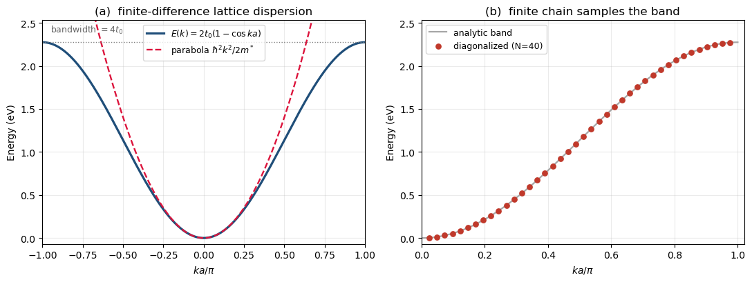
Figure 1. The lattice dispersion agrees with the continuum parabola near $k=0$ and has a finite bandwidth $4t_0$. A finite hard-wall chain does not create a different band; it samples that band at quantized wave numbers.

---

2. What a closed chain teaches us—and what it cannot teach us

Take $N$ physical sites and impose hard-wall conditions at two ghost points,

\[\psi_0=\psi_{N+1}=0.\]

The allowed modes are

\[k_na=\frac{n\pi}{N+1}, \qquad \psi_n(j)=\sqrt{\frac{2}{N+1}} \sin\!\left(\frac{n\pi j}{N+1}\right),\]

with energies

\[E_n=2t_0\left[1-\cos\!\left(\frac{n\pi}{N+1}\right)\right].\]

Direct diagonalization in the notebook agrees with this formula to $1.33\times10^{-15}\ \mathrm{eV}$, and the analytic eigenvectors satisfy $\lVert H\psi_n-E_n\psi_n\rVert<5.5\times10^{-16}\ \mathrm{eV}$.

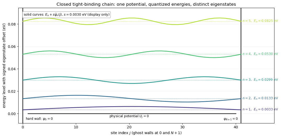
Figure 2. The vertical offset is only a display device: each signed eigenfunction is drawn around its own energy. The physical potential is $U_j=0$ between the two hard walls.

This closed problem is an essential check on the Hamiltonian, but it still contains no transport experiment. It has

• no right-moving incident population supplied by a left reservoir,
• no left-moving incident population supplied by a right reservoir,
• no place for probability to escape,
• and only discrete stationary levels.

For this real, time-reversal-symmetric one-dimensional chain, the hard-wall eigenstates can be chosen real. Their nearest-neighbor probability current vanishes. Adding more closed sites does not solve the conceptual problem; it merely delays the return from the artificial wall and makes the standing-wave level spacing denser.

To describe transport, the boundary condition—not merely the matrix size—must change.

---

3. A Green’s function is an energy-resolved response operator

Before opening the system, reinterpret the Schrödinger equation as a source-response problem. At a chosen energy, write

\[\big[(E+i\eta)I-H\big]\lvert\psi\rangle=\lvert s\rangle, \qquad \eta>0.\]

The source vector $\lvert s\rangle$ is a mathematical probe, not a reservoir occupation. The solution is

\[\lvert\psi\rangle=G^R(E)\lvert s\rangle, \qquad G^R(E)=\big[(E+i\eta)I-H\big]^{-1}. \tag{3}\]

Thus $G^R_{ab}$ is the amplitude observed at basis state $a$ in response to a unit source at basis state $b$. Because the matrix being inverted has units of energy, $G^R$ has units of inverse energy.

For a closed Hamiltonian with eigenstates $\lvert n\rangle$,

\[G^R(E)=\sum_n\frac{\lvert n\rangle\langle n\rvert}{E-E_n+i\eta}. \tag{4}\]

Equation (4) connects the eigenstate picture to an energy scan. Near $E_n$, the corresponding denominator becomes small and the response is large. The spectral function

\[A(E)=i\big(G^R-G^A\big), \qquad G^A=G^{R\dagger},\]

turns those poles into spectral weight, and the local density of states per spin is

\[\rho_j(E)=\frac{A_{jj}(E)}{2\pi}.\]

The spectral representation explains why a Green’s function contains more information than a list of eigenvalues. It retains one projector for every eigenstate:

\[P_n=\lvert n\rangle\langle n\rvert.\]

This projector preserves where the mode responds, while the denominator in eq. (4) determines at which energy that response becomes large. A Green’s function can therefore be evaluated at any probe energy, not only at an eigenvalue.

The same analytic structure survives in an open system, but a closed-system pole on the real axis generally moves into the complex-energy plane. Its real part gives the resonance position; its negative imaginary part gives escape-induced decay.

There is also a useful distinction between a pole and a peak. A pole belongs to the analytic continuation of $G^R$ into the complex plane. A peak is a feature seen on a real, finite-resolution energy scan.

Well-separated, weakly energy-dependent resonances make the two notions nearly interchangeable; overlapping resonances, thresholds, or rapidly varying self-energies do not.

For an isolated finite system, the exact $\eta\to0^+$ spectrum is a set of delta peaks. A finite plotting $\eta$ merely draws those peaks with visible width. It must not be confused with a physical lifetime.

Why insist on the plus sign in $E+i\eta$? In the time domain it gives a response only after the source is applied. In a lead it selects waves that leave the device, not waves mysteriously arriving from infinity. This analytic boundary condition is the meaning of the superscript $R$ in “retarded.”

---

4. Opening the system by eliminating a lead exactly

Before carrying the full matrix notation, consider the same algebra with two abstract blocks:

\[a_D\psi_D-\tau\psi_L=s_D, \qquad -\tau^\dagger\psi_D+a_L\psi_L=0.\]

The second equation says $\psi_L=a_L^{-1}\tau^\dagger\psi_D$. Substitution gives

\[\big(a_D-\tau a_L^{-1}\tau^\dagger\big)\psi_D=s_D.\]

Nothing has been discarded: the eliminated variable returns as the feedback term $\tau a_L^{-1}\tau^\dagger$. The Schur complement is exactly this substitution performed with matrices and operators.

Partition the one-particle basis into a finite device subspace $D$ and a lead subspace $L$:

\[H_{\mathrm{tot}}= \begin{pmatrix} H_D & \tau\\ \tau^\dagger & H_L \end{pmatrix}, \qquad \lvert\psi\rangle= \begin{pmatrix} \lvert\psi_D\rangle\\ \lvert\psi_L\rangle \end{pmatrix}. \tag{5}\]

Our convention is worth stating explicitly:

• $\tau=H_{DL}$ maps a lead amplitude into the device equation;
• $\tau^\dagger=H_{LD}$ maps a device amplitude into the lead equation;
• $g_L^R=[(E+i\eta)I_L-H_L]^{-1}$ is the Green’s function of the isolated lead.

Lowercase $g_L^R$ must not be confused with the $G_{LL}^R$ block of the already coupled full Green’s function; the latter also contains excursions through the device. The matrix dimensions and units provide a useful check:

\[(N_D\!\times\!N_L)\, (N_L\!\times\!N_L)\, (N_L\!\times\!N_D) \longrightarrow N_D\!\times\!N_D,\]

and $(\mathrm{eV})(\mathrm{eV}^{-1})(\mathrm{eV})=\mathrm{eV}$, as required for a term added to $H_D$.

For a source applied only in the device, the block equation is

\[\begin{aligned} \big[(E+i\eta)I_D-H_D\big]\psi_D-\tau\psi_L&=s_D,\\ -\tau^\dagger\psi_D+ \big[(E+i\eta)I_L-H_L\big]\psi_L&=0. \end{aligned} \tag{6}\]

The second row can be solved without approximation:

\[\psi_L=g_L^R\tau^\dagger\psi_D. \tag{7}\]

Substitute this expression into the first row:

\[\left[(E+i\eta)I_D-H_D- \underbrace{\tau g_L^R\tau^\dagger}_{\Sigma_L^R(E)} \right]\psi_D=s_D. \tag{8}\]

The lead self-energy is therefore

\[\boxed{\Sigma_L^R(E)=\tau g_L^R(E)\tau^\dagger}. \tag{9}\]

Read the product from right to left. An amplitude at the device boundary goes from $D$ to $L$ through $\tau^\dagger$, propagates through the isolated lead with $g_L^R$, and returns from $L$ to $D$ through $\tau$. The self-energy is the complete leave-propagate-return amplitude.

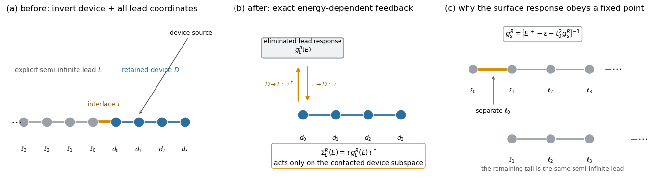
Figure 3. Panel (a) shows the explicit device-plus-lead coordinates. Panel (b) retains only the device but preserves the exact feedback $\Sigma_L^R$. Panel (c) previews why a uniform semi-infinite lead has a recursive surface response.

Several common misunderstandings disappear if we say precisely what is exact.

• The equality is between the device block of the full resolvent and the inverse in eq. (8).
• It is not a claim that the full Hermitian Hamiltonian equals a smaller non-Hermitian Hamiltonian.
• The elimination is exact for the chosen single-particle Hamiltonian and partition.
• The resulting operator is energy dependent because the eliminated lead has its own dynamics.
• It can be non-Hermitian on the real axis because an outgoing wave can escape from the retained subspace.

Another way to read the same result is through repeated excursions. Let

\[g_D^R=[(E+i0^+)I_D-H_D]^{-1}\]

be the disconnected-device resolvent. Define the total lead self-energy by

\[\Sigma^R\equiv\Sigma_L^R+\Sigma_R^R,\]

so it contains the feedback from every eliminated lead. The Dyson equation is then

\[G^R=g_D^R+g_D^R\Sigma^RG^R,\]

or, as a formal series,

\[G^R =g_D^R +g_D^R\Sigma^Rg_D^R +g_D^R\Sigma^Rg_D^R\Sigma^Rg_D^R+\cdots.\]

Each $\Sigma^R$ represents one complete leave-propagate-return event; the inverse in eq. (10) resums any number of such events. Thus, “eliminating the lead” does not mean allowing the electron to visit it only once. It means summing the lead’s linear response to all orders without retaining its coordinates explicitly.

With both contacts eliminated, the finite matrix we actually invert is

\[G^R(E)= \left[ (E+i0^+)I_D-H_D-\Sigma_L^R(E)-\Sigma_R^R(E) \right]^{-1}. \tag{10}\]

The notebook tests the Schur-complement identity by comparing eq. (10) against the device block of a direct device-plus-finite-lead inverse. The maximum difference is $3.48\times10^{-15}\ \mathrm{eV}^{-1}$.

Code: the finite-lead Schur-complement check

g_L = np.linalg.inv(z * np.eye(N_L) - H_L)
Sigma_L = tau @ g_L @ tau.conj().T

G_D_schur = np.linalg.inv(
    z * np.eye(N_D) - H_D - Sigma_L
)

H_full = np.block([
    [H_D,          tau],
    [tau.conj().T, H_L],
])
G_full = np.linalg.inv(z * np.eye(N_D + N_L) - H_full)
G_D_projected = G_full[:N_D, :N_D]

print(np.max(np.abs(G_D_projected - G_D_schur)))

---

5. Why one surface Green’s function contains an infinite lead

For a one-orbital contact, the device boundary $\lvert d_0\rangle$ touches only the lead surface site $\lvert\ell_0\rangle$:

\[\tau=-t_0\lvert d_0\rangle\langle\ell_0\rvert.\]

Substituting this sparse coupling into eq. (9) gives

\[\Sigma_L^R =t_0^2\lvert d_0\rangle \underbrace{\langle\ell_0\rvert g_L^R\lvert\ell_0\rangle}_{g_s^R(E)} \langle d_0\rvert.\]

Although $g_L^R$ is an infinite matrix, multiplication by $\tau$ on both sides selects only one surface-to-surface element:

\[g_s^R(E)=\langle\ell_0\rvert g_L^R(E)\lvert\ell_0\rangle.\]

Suppose the lead is uniform, semi-infinite, has on-site energy $\varepsilon$, and nearest-neighbor hopping $-t_0$. In the finite-difference wire of section 1, $\varepsilon=2t_0+U_{\mathrm{lead}}$; a clean lead with $U_{\mathrm{lead}}=0$ therefore still has the band $[0,4t_0]$.

Remove the surface site $\ell_0$. The remaining chain beginning at $\ell_1$ is identical to the original chain after relabeling. Its new surface Green’s function is therefore the same $g_s^R$.

Applying the same elimination once gives the fixed-point equation

\[g_s^R(E)= \frac{1}{E+i0^+-\varepsilon-t_0^2g_s^R(E)}. \tag{11}\]

The same self-similarity appears as an infinite continued fraction:

\[g_s^R= \cfrac{1}{E^+-\varepsilon- \cfrac{t_0^2}{E^+-\varepsilon- \cfrac{t_0^2}{\ddots}}}.\]

Multiplication produces a quadratic,

\[t_0^2(g_s^R)^2- (E+i0^+-\varepsilon)g_s^R+1=0,\]

with algebraic roots

\[g_\pm(E)= \frac{E+i0^+-\varepsilon \ \pm\ \sqrt{(E+i0^+-\varepsilon)^2-4t_0^2}} {2t_0^2}. \tag{12}\]

Solving the quadratic is not the end of the problem: only one root is retarded. We denote that selected physical root by $g_s^R$. It is fixed by three equivalent requirements.

1. It is analytic when $\operatorname{Im}E>0$ and has $\operatorname{Im}g_s^R\le0$ on the real axis.
2. It behaves as $g_s^R\sim1/E$ far from the band.
3. Outside the band, the corresponding spatial solution decays into the lead rather than growing toward infinity.

Inside the lead band, parameterize energy as

\[E=\varepsilon-2t_0\cos ka, \qquad 0<ka<\pi.\]

For the present hopping convention,

\[g_s^R(E)=-\frac{e^{ika}}{t_0}. \tag{13}\]

Here each lead has its own local site coordinate $n=0,1,\ldots$ increasing away from the device. Equation (13) is therefore outward-going in either lead: it corresponds to global $+k$ on the right and global $-k$ on the left.

It is useful to define $q=-t_0g_s^R$. Then $q=e^{ika}$ lies on the upper unit semicircle in the ideal $\eta\to0^+$ limit. Outside the band the physical continuation has $\lvert q\rvert<1$; the reciprocal quadratic root has $\lvert q\rvert>1$ and grows into the lead.

def surface_green_scalar(E, t0, eps_lead, eta=1e-9):
    b = (E + 1j * eta) - eps_lead
    disc = np.sqrt(b * b - 4.0 * t0 * t0 + 0j)
    roots = ((b + disc) / (2.0 * t0**2),
             (b - disc) / (2.0 * t0**2))

    # In the propagating band, the retarded root has Im(g_s) < 0.
    for g in roots:
        if g.imag < 0:
            return g

    # At eta=0 outside the band, choose the decaying/asymptotic root.
    return min(roots, key=lambda g: abs(t0 * g))

def lead_self_energy_scalar(E, t0, eps_lead, eta=1e-9):
    """Matched endpoint: sigma^R = t0^2 g_s^R."""
    return t0**2 * surface_green_scalar(E, t0, eps_lead, eta)

For a matched interface hopping $\tau=-t_0$, the scalar endpoint self-energy is

\[\sigma^R=t_0^2g_s^R=-t_0e^{ika} =\underbrace{-t_0\cos ka}_{\lambda(E)} -\frac{i}{2}\underbrace{2t_0\sin ka}_{\gamma(E)}. \tag{14}\]

The real part $\lambda=\operatorname{Re}\sigma^R$ shifts the boundary resonance condition. The positive broadening

\[\gamma=-2\operatorname{Im}\sigma^R\]

measures coupling to propagating escape channels. In matrix form,

\[\Gamma_\alpha =i\left(\Sigma_\alpha^R-\Sigma_\alpha^A\right) \succeq0. \tag{15}\]

Here $\Sigma_\alpha^A=\Sigma_\alpha^{R\dagger}$. For a matrix, the relevant “imaginary part” is the anti-Hermitian part

\[\operatorname{Im}_{H}X=\frac{X-X^\dagger}{2i}, \qquad \Gamma_\alpha=-2\operatorname{Im}_{H}\Sigma_\alpha^R.\]

This is not generally the same as taking the ordinary scalar imaginary part element by element. For the single scalar endpoint $\sigma^R$ used here, the two notions coincide.

For a general interface hopping $t_c$, the robust statement is

\[\gamma=2\pi\lvert t_c\rvert^2\rho_s, \qquad \rho_s=-\frac{1}{\pi}\operatorname{Im}g_s^R,\]

where $\rho_s$ is the surface, not bulk, density of states. The additional identity $\gamma=\hbar\lvert v\rvert/a$ holds for the matched contact $t_c=t_0$ used here; it should not be promoted to a universal formula for arbitrary interfaces.

The word “surface” matters in one dimension. From eq. (13), the endpoint spectral density inside the band is

\[\rho_s(E)=\frac{\sin ka}{\pi t_0}.\]

It vanishes at the band edges. By contrast, the translationally invariant bulk density of states per site is

\[\rho_{\mathrm{bulk}}(E) =\frac{1}{2\pi t_0\lvert\sin ka\rvert},\]

and diverges there. There is no contradiction. The bulk DOS counts how densely the allowed wave numbers crowd in energy, whereas the surface DOS also contains the weight of those modes on the endpoint orbital. Open-chain eigenmodes have small endpoint amplitude near a band edge, and that boundary weight cancels the bulk van Hove divergence.

For the matched scalar contact, the group velocity

\[v(k)=\frac{1}{\hbar}\frac{dE}{dk} =\frac{2t_0a}{\hbar}\sin ka\]

immediately gives $\gamma=2t_0\sin ka=\hbar\lvert v\rvert/a$. The same $\sin ka$ that closes the surface coupling at a band edge also drives the group velocity to zero.

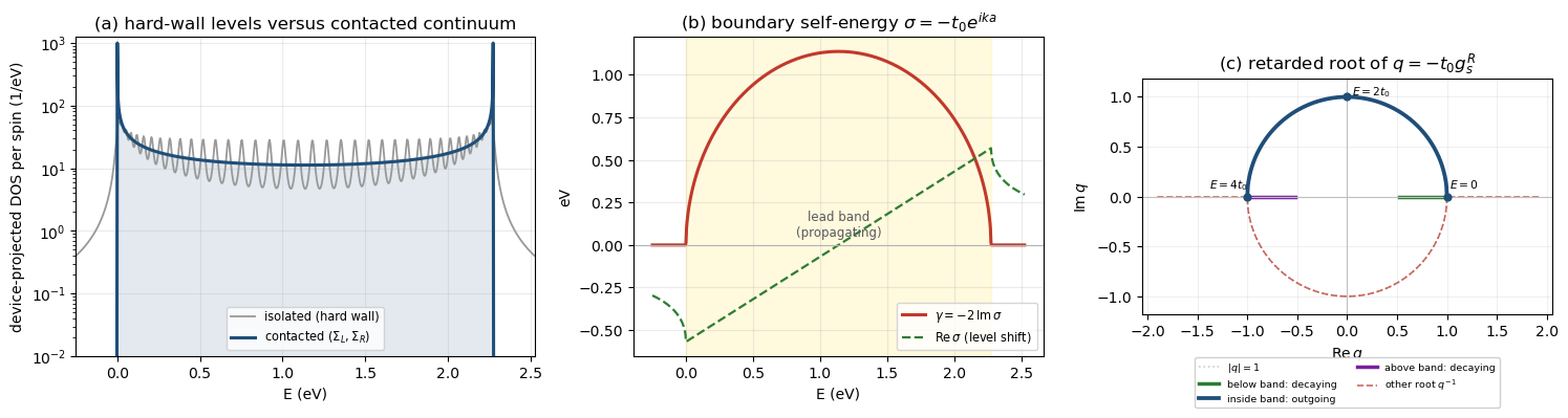
Figure 4. Opening the chain turns discrete hard-wall levels into a continuum over the lead band. The real self-energy shifts levels, the broadening closes outside the propagating band, and the complex-$q$ plot makes the retarded root choice geometric.

Notice what does not happen outside the band. The broadening vanishes because there is no propagating escape channel, but the real self-energy generally remains nonzero because the lead still supports an evanescent boundary response.

A separate device may also host a true bound state outside both lead continua; its occupation is not determined by the two contact Fermi functions alone.

---

6. From the open-device Green’s function to transmission

We now have every ingredient required to ask a transport question. At each energy:

1. compute the two lead surface Green’s functions;
2. embed their self-energies on the contacted device orbitals;
3. form $\Gamma_L$ and $\Gamma_R$;
4. invert the finite open-device operator to obtain $G^R$;
5. construct spectral functions and transmission.

The available device spectral weight is

\[A(E)=i(G^R-G^A). \tag{16}\]

Within the continuum generated by the contacts and in the $\eta\to0^+$ limit,

\[A=A_L+A_R, \qquad A_\alpha=G^R\Gamma_\alpha G^A. \tag{17}\]

$A_L$ is the device spectral weight associated with scattering states supplied from the left contact; $A_R$ is the analogous right-contact contribution. Neither contains a Fermi function yet. They answer where states are available, not whether those states are occupied.

The qualification in the previous paragraph matters. At finite numerical $\eta$,

\[i(G^R-G^A) =G^R\big(\Gamma_L+\Gamma_R+2\eta I\big)G^A.\]

The $2\eta I$ term is a regulator, not a third contact. A true bound state with $\Gamma_L=\Gamma_R=0$ also requires an occupation rule beyond the two ideal reservoirs.

6.1 Why the Caroli trace is a probability

The coherent transmission is

\[\boxed{ T(E)=\operatorname{Tr} \left[\Gamma_LG^R\Gamma_RG^A\right] }. \tag{18}\]

To expose the absolute-square structure, define

\[X=\Gamma_L^{1/2}G^R\Gamma_R^{1/2}.\]

Cyclicity of the trace gives

\[T=\operatorname{Tr}(XX^\dagger)\ge0.\]

Thus $T$ is a sum of squared, contact-weighted propagation amplitudes between channels. For a passive coherent device attached to ideal leads, the corresponding transmission eigenvalues lie between zero and one.

The matrix order in eq. (18) means: couple to one contact, propagate, couple to the other, and multiply by the conjugate process. The trace sums the contacted channels.

For the present single-channel chain,

\[\Gamma_L=\gamma_L\lvert1\rangle\langle1\rvert, \qquad \Gamma_R=\gamma_R\lvert N\rangle\langle N\rvert.\]

Substituting those rank-one matrices into eq. (18) collapses the trace:

\[T(E)=\gamma_L\gamma_R\lvert G^R_{1N}\rvert^2. \tag{19}\]

The two endpoint broadenings normalize injection and collection to lead flux; $G^R_{1N}$ is the amplitude to propagate between the endpoints. That is why the result is dimensionless even though $G^R$ has units $\mathrm{eV}^{-1}$ and each $\gamma$ has units eV.

The central implementation is short:

def retarded_greens_function(E, H, Sigma_L, Sigma_R, eta=1e-9):
    I = np.eye(H.shape[0], dtype=complex)
    return np.linalg.inv(
        (E + 1j * eta) * I - H - Sigma_L - Sigma_R
    )

def broadening(Sigma):
    return 1j * (Sigma - Sigma.conj().T)

def transmission(Gamma_L, GR, Gamma_R):
    GA = GR.conj().T
    return np.trace(Gamma_L @ GR @ Gamma_R @ GA).real

6.2 The potential and the Hamiltonian are related, but not identical

Before looking at transmission, it is useful to draw both the spatial input and the matrix that the code actually inverts. The notebook compares a clean device with a six-site barrier of height $V_b=0.60\ \mathrm{eV}$.

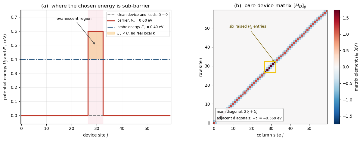
Figure 5. The barrier raises only the selected diagonal entries from $2t_0$ to $2t_0+V_b$. The off-diagonal hopping remains $-t_0$. The orange marker $E_{\mathrm{probe}}=0.400\ \mathrm{eV}$ lies below the local barrier bottom and is used later to visualize evanescent tunneling.

Within a locally uniform region of potential energy $U$, the lattice dispersion is

\[E=U+2t_0(1-\cos ka).\]

Real $k$ exists only for

\[U\le E\le U+4t_0.\]

Thus $E<V_b$ means the wave number inside this barrier is complex. It does not mean the wavefunction must be zero there. A finite evanescent segment can connect the propagating solutions on its two sides. Writing $k=i\kappa$ near the lower local band gives

\[\cosh(\kappa a)=1+\frac{U-E}{2t_0}.\]

The exact state inside a finite barrier is a boundary-matched combination of growing and decaying evanescent pieces, not a single exponential. Its LDOS envelope therefore need not decrease perfectly monotonically on every site.

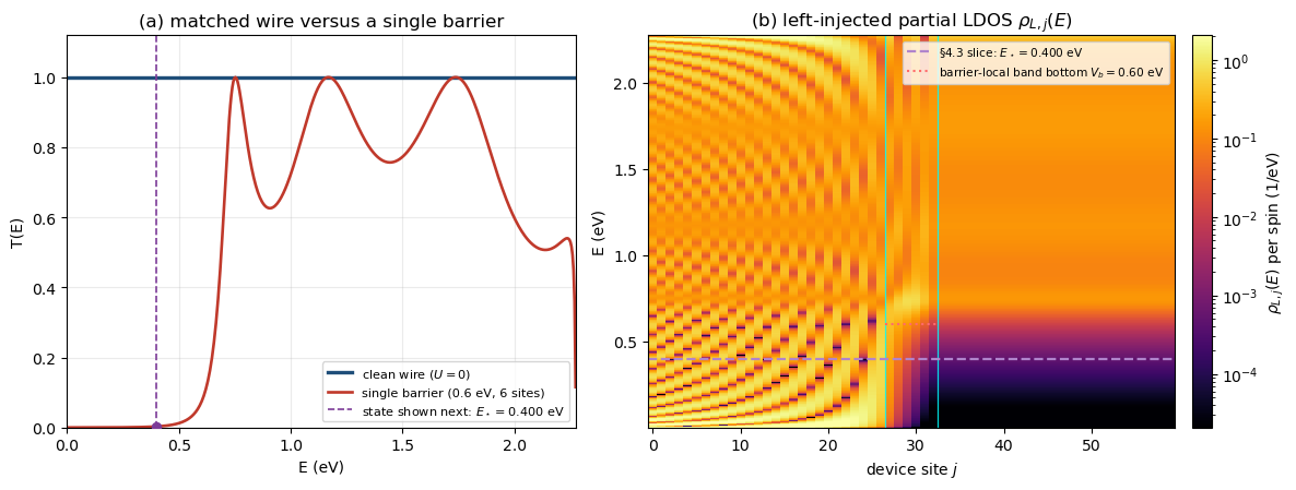
Figure 6. A device identical to its leads has no interface and therefore $T(E)=1$ inside the open band, apart from the singular band-edge limit. The barrier produces reflection, energy-dependent transmission, and a spatially structured left-injected partial LDOS $[A_L]_{jj}/(2\pi)$. This is available spectral weight before multiplication by $f_L$; it is not the total occupied density.

The matched-wire result is an especially strong unit test. It gives

\[\mathcal G_0=\frac{2e^2}{h}=77.4809\ \mu\mathrm{S}, \qquad R_0=12.9064\ \mathrm{k}\Omega,\]

and the notebook obtains $0.999999997\le T\le1.000000000$ across the sampled interior of the band. A sign error in the self-energy or a misplaced endpoint index usually destroys this check immediately.

The conductance quantum follows from the finite-bias current rather than being inserted as a normalization. For a small electrochemical-potential difference $\Delta\mu=e\,\Delta V$,

\[f_L(E)-f_R(E) \simeq-\frac{\partial f}{\partial E}\,\Delta\mu.\]

At zero temperature, $-\partial f/\partial E$ becomes $\delta(E-E_F)$. Linearizing the Landauer current that will be derived in eq. (27) then gives

\[\mathcal G =\left.\frac{dI}{dV}\right\rvert_{V=0} =\frac{2e^2}{h}T(E_F).\]

The factor $2e^2/h$ is therefore the one-channel, spin-degenerate conductance scale. A clean matched wire reaches it because its scattering probability is unity, not because the plotted transmission was divided by a convenient constant.

6.3 What tunneling looks like in real space

For the rank-one left contact define the device-projected, contact-normalized spectral amplitude

\[\lvert\psi_L(E)\rangle =G^R(E)\sqrt{\gamma_L(E)}\lvert1\rangle. \tag{20}\]

It is not a unit-normalized bound-state wavefunction. Its units are $\mathrm{eV}^{-1/2}$, and it factorizes the partial spectral function:

\[A_L=\lvert\psi_L\rangle\langle\psi_L\rvert.\]

Consequently,

\[\rho_{L,j}(E)=\frac{\lvert\psi_{L,j}(E)\rvert^2}{2\pi}\]

is the left-contact contribution to the LDOS per spin. The directed spectral flux on bond $j\to j+1$ is

\[\mathcal J_{j\to j+1}^{(L)}(E) =-2\operatorname{Im} \left[H_{j,j+1}\psi_{L,j+1}\psi_{L,j}^*\right]. \tag{21}\]

For coherent steady propagation, this flux is independent of $j$ and equals the transmission in the present reciprocal single-channel model.

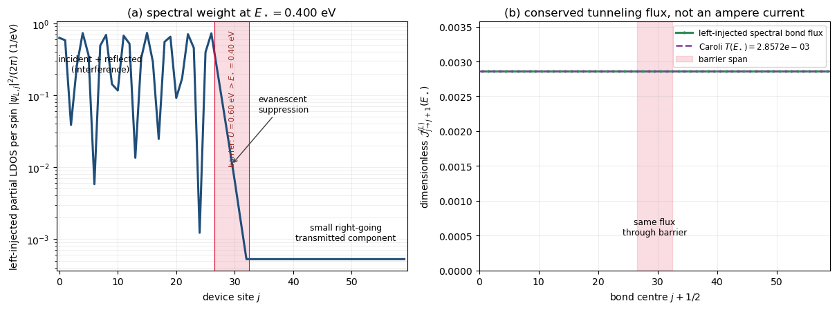
Figure 7. At $E_{\mathrm{probe}}=0.400\ \mathrm{eV}$, the partial LDOS is strongly suppressed through the barrier, yet a nonzero transmitted component survives. The spatial weight changes dramatically while the directed flux stays constant at $T=2.8572\times10^{-3}$.

This figure is the cleanest answer to the phrase “the particle tunnels through the barrier.” A stationary scattering state is matched across the entire structure. Its amplitude is evanescent in the classically forbidden segment, but its phase relation carries one conserved, small flux.

At equilibrium, an equal right-injected contribution cancels the left-injected flux. An electrical current appears only after the reservoirs occupy the two directions differently.

---

7. Nonequilibrium requires occupation information

$G^R$, $A_L$, $A_R$, and $T$ describe the open spectrum and propagation. If the Hamiltonian and contact structure are fixed, they do not change merely because the reservoirs are filled differently.

The population of reservoir $\alpha$ is

\[f_\alpha(E)= \frac{1}{1+\exp[(E-\mu_\alpha)/(k_BT_\alpha)]}. \tag{22}\]

At equilibrium $f_L=f_R=f$, so one Fermi function fills the contact-generated spectrum. Out of equilibrium, no single Fermi function describes the device interior. The in-scattering self-energy is

\[\Sigma^{\mathrm{in}}(E) =\Gamma_L(E)f_L(E)+\Gamma_R(E)f_R(E). \tag{23}\]

The occupied-state correlation function is

\[\begin{aligned} G^n(E) &=G^R\Sigma^{\mathrm{in}}G^A\\ &=A_Lf_L+A_Rf_R. \end{aligned} \tag{24}\]

There is a useful source-covariance interpretation of this equation. If the linear response is $\lvert\psi\rangle=G^R\lvert s\rangle$ and incoherent injection has source correlation $\langle ss^\dagger\rangle=\Sigma^{\mathrm{in}}$, then

\[\langle\psi\psi^\dagger\rangle =G^R\Sigma^{\mathrm{in}}G^A.\]

This is the intuitive core of the Keldysh relation: propagate the covariance of the injected amplitudes through the retarded and advanced response operators.

This post uses the convention

\[G^n=-iG^<.\]

Keeping that convention explicit prevents a common sign error when formulas from different texts are mixed.

The conceptual separation is now complete:

A_alpha(E): where contact-alpha scattering states have spectral weight
f_alpha(E): whether contact alpha occupies those states
G^n(E):     the resulting occupied spectral weight inside the device

The corresponding code mirrors the algebra:

def in_scattering(Gamma_L, Gamma_R, f_L, f_R):
    return Gamma_L * f_L + Gamma_R * f_R

def electron_correlation(GR, Sigma_in):
    return GR @ Sigma_in @ GR.conj().T

def bond_current_integrand(H, Gn, i):
    return -2.0 * np.imag(H[i, i + 1] * Gn[i + 1, i])

The site occupation, including twofold spin degeneracy, is

\[n_j=2\int\frac{dE}{2\pi}[G^n(E)]_{jj}. \tag{25}\]

The current across a nearest-neighbor bond is

\[I_{j\to j+1} =-\frac{2e}{h}\int dE\, 2\operatorname{Im} \left[H_{j,j+1}G^n_{j+1,j}(E)\right]. \tag{26}\]

Why does an off-diagonal element appear? The occupation of site $j$ is $\hat n_j=c_j^\dagger c_j$. Applying the Heisenberg equation to the hopping Hamiltonian gives a lattice continuity equation,

\[\frac{d\langle\hat n_j\rangle}{dt} +\mathcal J_{j\to j+1} -\mathcal J_{j-1\to j}=0.\]

Only hopping terms that connect $j$ to a neighbor fail to commute with $\hat n_j$. Their expectation values are coherences such as $\langle c_j^\dagger c_{j+1}\rangle$, not diagonal populations.

In the present convention that coherence is represented by $G^n_{j+1,j}$, and its imaginary part distinguishes a traveling phase relation from a standing one.

This is why the diagonal of $G^n$ gives particle occupation while the first off-diagonal gives bond flow. The electronic charge associated with an occupation is obtained only after multiplying by $-e$.

Here $\mathcal J$ denotes particle-number flux in the lattice continuity equation; the electrical-current convention and its charge prefactor enter eq. (26).

In the exact $\eta\to0^+$ stationary coherent problem there is no accumulation in any interior site. The accumulation term in the continuity equation therefore vanishes, and every internal bond carries the same integrated current.

A finite numerical $\eta$ behaves like a weak distributed absorber and can produce the tiny drift reported below. Any spread larger than that controlled regulator effect signals inadequate energy resolution, inconsistent indices or signs, a missing source/sink term, or a numerical failure.

There are two different factors of two in this discussion. The factor in $2e/h$ is spin degeneracy. The factor inside the integrand comes from combining a hopping term with its Hermitian conjugate in the continuity equation. Counting both as spin would double the current incorrectly.

7.1 Recovering Landauer from the correlation function

The left-terminal current is injection minus escape. In the next expression, the first term is occupied spectral weight injected by the left contact, while the second is the part of the already occupied device spectrum that escapes back through that contact:

\[I_L=\frac{2e}{h}\int dE\, \operatorname{Tr} \left[\Sigma_L^{\mathrm{in}}(A_L+A_R)-\Gamma_LG^n\right].\]

Insert $\Sigma_L^{\mathrm{in}}=\Gamma_Lf_L$ and $G^n=A_Lf_L+A_Rf_R$. The $A_Lf_L$ terms cancel, leaving

\[I=\frac{2e}{h}\int dE\, T(E)[f_L(E)-f_R(E)]. \tag{27}\]

This is the Landauer current. Transmission alone is not a current: it must be weighted by the imbalance of incident populations and integrated over energy.

The notebook stores energy grids in eV while $h$ is in joule-seconds. Therefore the numerical prefactor is

\[\frac{2e}{h}J_{\mathrm{per\,eV}}, \qquad J_{\mathrm{per\,eV}}=1.602176634\times10^{-19}\ \mathrm{J/eV}.\]

The symbol $e>0$ denotes the magnitude of the elementary charge. The notebook calls $I>0$ the left-to-right electron-flow direction when $f_L>f_R$. Conventional signed charge current points oppositely because an electron carries charge $-e$.

---

8. Example A: a fixed spectrum filled by two reservoirs

The first resonant-tunneling example separates propagation from population as cleanly as possible. The device contains two barriers of height $0.40\ \mathrm{eV}$ around a 16-site well. The device Hamiltonian, both lead bands, and all retarded self-energies remain fixed while $\mu_L$ and $\mu_R$ are placed on opposite sides of one resonance.

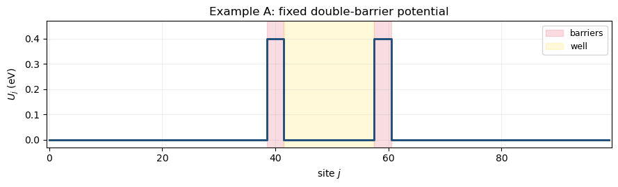
Figure 8. The plotted line is $U_j$, not the Hamiltonian diagonal $2t_0+U_j$. Openness enters later through endpoint self-energies; it is not drawn as an imaginary potential in the device interior.

8.1 From a closed-well level to an open resonance

If the two barriers were infinitely high, the well would have discrete bound levels. Finite barriers couple those modes to left- and right-going continua.

For an isolated resonance $r$, let $\lvert\phi_r\rangle$ be the normalized, device-region, closed-well-like orbital associated with that resonance. If the contact self-energies vary slowly across its width, the projected partial linewidths are approximately

\[\Gamma_{\alpha,r}\simeq \langle\phi_r\rvert\Gamma_\alpha(E_r)\lvert\phi_r\rangle, \qquad \alpha=L,R.\]

Under the same isolated-resonance approximation, the analytically continued device Green’s function has a pole near

\[\mathcal E_r\simeq E_r-\frac{i}{2}\Gamma_r, \qquad \Gamma_r\simeq\Gamma_{L,r}+\Gamma_{R,r}.\]

Here $E_r$ is the contact-shifted resonance energy. This complex pole is not an extra complex eigenvalue of the full Hermitian device-plus-leads Hamiltonian; it belongs to the analytic continuation of the projected open-device response. Strongly energy-dependent or overlapping resonances require going beyond this simple projection.

Near an isolated resonance, the transmission has the Breit-Wigner form

\[T(E)\approx \frac{\Gamma_{L,r}\Gamma_{R,r}} {(E-E_r)^2+(\Gamma_r/2)^2}. \tag{28}\]

At the resonance energy,

\[T(E_r)= \frac{4\Gamma_{L,r}\Gamma_{R,r}} {(\Gamma_{L,r}+\Gamma_{R,r})^2}.\]

This reaches one for symmetric left and right coupling. Even if either barrier is strongly reflecting away from resonance, repeated phase-coherent reflections in the well can add constructively, much like a Fabry-Pérot cavity.

The probability lifetime is approximately

\[t_{\mathrm{life},r}\simeq\frac{\hbar}{\Gamma_r}.\]

$\Gamma_r$ is an energy linewidth; the decay rate is $\Gamma_r/\hbar$. Using a distinct symbol $t_{\mathrm{life},r}$ avoids confusing the lifetime with the interface coupling matrix $\tau$.

The resolved sub-barrier resonances in the notebook occur at

\[E_r\approx 0.0639,\ 0.1413,\ 0.2453,\ 0.3713\ \mathrm{eV},\]

with an additional resolved feature near $0.5146\ \mathrm{eV}$. We select

\[E_{\mathrm{res}}=0.1413\ \mathrm{eV}, \qquad \mu_L=0.201\ \mathrm{eV}, \qquad \mu_R=0.081\ \mathrm{eV}, \qquad k_BT=0.005\ \mathrm{eV}=5\ \mathrm{meV}.\]

The last value corresponds to about $58\ \mathrm{K}$ and is an energy scale, not another transmission parameter. The resonance list is the set of detected and numerically refined peaks on this scan, not a theorem that no other arbitrarily narrow feature exists.

8.2 Available spectrum is not occupied spectrum

Project the two partial spectral functions onto the well region $W$:

\[\rho_{W,L}(E)=\frac{1}{2\pi}\sum_{j\in W}[A_L(E)]_{jj}, \qquad \rho_{W,R}(E)=\frac{1}{2\pi}\sum_{j\in W}[A_R(E)]_{jj}.\]

Those functions describe available left- and right-connected well states. Occupied spectral weight is instead

\[f_L\rho_{W,L}+f_R\rho_{W,R}.\]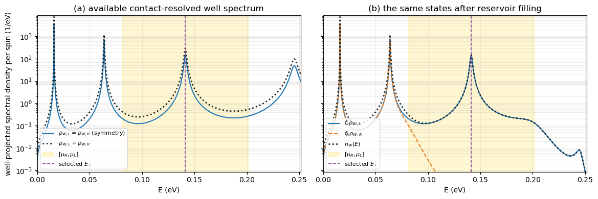

Figure 9. The same fixed resonances are available to both contacts. The chemical potentials change only how the two reservoirs fill that spectrum. This is the most direct visual meaning of $G^n=A_Lf_L+A_Rf_R$.

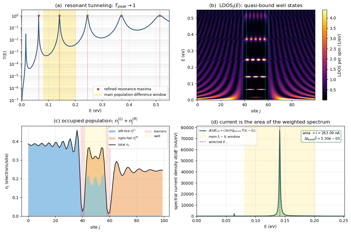
Figure 10. Panel (a) shows the fixed transmission spectrum and the main occupation window. Panel (b) reveals quasi-bound well modes in the LDOS. Panel (c) separates left-fed and right-fed occupation. Panel (d) emphasizes that current is the area of $dI/dE$, not simply the height of a transmission peak.

Resolving those areas is a numerical part of the physics. A uniform energy mesh can miss a narrow resonance or poorly sample the integrable one-dimensional threshold structure.

The notebook therefore joins a geometric mesh close to the emitter band bottom to a fine linear mesh over the occupied range. It also refines every candidate transmission maximum locally instead of reporting the nearest plotted grid point as the resonance energy.

For a nonuniform mesh $E_0<\cdots<E_{M-1}$, the trapezoidal rule can be written as $\int dE\,F(E)\simeq\sum_iw_iF(E_i)$ with

\[w_0=\frac{E_1-E_0}{2},\qquad w_i=\frac{E_{i+1}-E_{i-1}}{2},\qquad w_{M-1}=\frac{E_{M-1}-E_{M-2}}{2}.\]

Writing the weights explicitly makes it difficult to accidentally integrate an array as though its samples were equally spaced:

E = np.unique(np.concatenate((
    np.geomspace(1e-10, 1e-3, 400, endpoint=False),
    np.linspace(1e-3, mu_L + 0.05, 3000),
)))
w = np.empty_like(E)
w[0], w[-1] = 0.5 * (E[1] - E[0]), 0.5 * (E[-1] - E[-2])
w[1:-1] = 0.5 * (E[2:] - E[:-2])

n_per_spin += w[iE] * np.diag(Gn).real / (2.0 * np.pi)
n_site = 2.0 * n_per_spin                 # apply spin degeneracy once
I = current_prefactor_A_per_eV * np.sum(w * T_E * (f_L - f_R))

Here current_prefactor_A_per_eV already contains the spin factor and the eV-to-joule conversion; multiplying by another two would be an error. The same energy samples and the same weights are used for density, bond current, and terminal current, so discrepancies among them remain meaningful diagnostics rather than quadrature artifacts.

The independent current calculations agree:

\[I_{\mathrm{Landauer}}=263.0891\ \mathrm{nA},\]

while the mean bond current is $263.0900\ \mathrm{nA}$ with relative spatial spread $5.30\times10^{-5}$. The contact decomposition $n=n_L+n_R$ closes to $3.0\times10^{-15}$ relative error. Independently, integrating the occupied well spectrum and summing the site occupations both give $4.882464787$ electrons for this spin-degenerate model.

The lesson of Example A is narrow but foundational:

Changing f_L and f_R changes occupation and current.
It does not, by itself, change G^R if H_D and the lead self-energies stay fixed.

---

9. Example B: voltage-dependent resonances and NDR

A real voltage can also reshape the one-particle potential and shift a contact band. Example B represents that effect with an imposed electron potential-energy profile $U=-e\phi$ corresponding to an assumed linear electrostatic drop; it is not a self-consistent Poisson solution.

This is a separate, narrower-well device with 90 sites, $0.45\ \mathrm{eV}$ barriers, and an 8-site well.

The resolved zero-bias resonances are

\[E_r(0)\approx0.0504,\ 0.1946,\ 0.4109\ \mathrm{eV}.\]

The operating point deliberately puts the Fermi level $15\ \mathrm{meV}$ below the lowest resonance:

\[E_F=E_1(0)-0.015\ \mathrm{eV}=0.0354\ \mathrm{eV}, \qquad k_BT=0.003\ \mathrm{eV}\quad(T\approx35\ \mathrm{K}).\]

Thus the lowest resonance begins $15\ \mathrm{meV}$ above the emitter Fermi level and can be swept into, then out of, effective alignment.

The electron potential-energy shift is prescribed as

\[U_j^{\mathrm{bias}}(V) =-eV\frac{j}{N-1}.\]

Because the arrays store energy in eV, the numerical implementation is simply

\[U_j^{\mathrm{bias}}[\mathrm{eV}] =-V[\mathrm{V}]\frac{j}{N-1}. \tag{29}\]

Multiplying the eV array by the SI charge again would be a unit error. In physical energy units, the right lead and its reservoir move consistently as $\varepsilon_R(V)=\varepsilon_L-eV$ and $\mu_R(V)=E_F-eV$. When energies are recorded numerically in eV and $V$ in volts, this becomes

\[\varepsilon_R[\mathrm{eV}]=\varepsilon_L[\mathrm{eV}]-V[\mathrm{V}], \qquad \mu_R[\mathrm{eV}]=E_F[\mathrm{eV}]-V[\mathrm{V}], \qquad \mu_L[\mathrm{eV}]=E_F[\mathrm{eV}]. \tag{30}\]

Thus $\mu_R$ remains at the same filling relative to the shifted right-lead band bottom. The voltage is not applied twice.

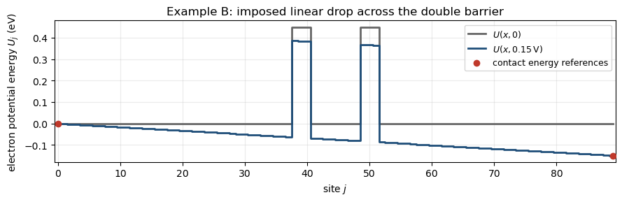
Figure 11. The linear ramp is an input assumption, not the output of a Poisson solver. It tilts the well and barriers while the collector energy reference shifts downward.

9.1 Why the sweep can be reduced from $O(N^3)$ to $O(N)$ per point

The voltage-energy map needs many evaluations of $T(E,V)$. A dense inverse costs $O(N^3)$, but the device operator

\[\mathcal A(E,V) =(E+i0^+)I-H_D(V)-\Sigma_L^R-\Sigma_R^R\]

is tridiagonal. Endpoint contacts require only $G^R_{1N}$. Solve

\[\mathcal A\mathbf x=\mathbf e_N;\]

then $x_1=G^R_{1N}$. A banded solve obtains this element in $O(N)$ work.

Code: endpoint transmission with a tridiagonal solve

from scipy.linalg import solve_banded

def transmission_fast(E, N, t0, U, eps_L, eps_R, eta=1e-9):
    sigma_L = lead_self_energy_scalar(E, t0, eps_L, eta)
    sigma_R = lead_self_energy_scalar(E, t0, eps_R, eta)

    diag = ((E + 1j * eta) - (2.0 * t0 + U)).astype(complex)
    diag[0]  -= sigma_L
    diag[-1] -= sigma_R

    # A has +t0 on both off-diagonals because H has -t0.
    ab = np.zeros((3, N), dtype=complex)
    ab[0, 1:] = t0
    ab[1, :] = diag
    ab[2, :-1] = t0

    rhs = np.zeros(N, dtype=complex)
    rhs[-1] = 1.0
    last_column = solve_banded((1, 1), ab, rhs)

    gamma_L = -2.0 * sigma_L.imag
    gamma_R = -2.0 * sigma_R.imag
    return (gamma_L * gamma_R * abs(last_column[0])**2).real

At $E=0.09\ \mathrm{eV}$, the fast and dense calculations differ by only $4.61\times10^{-19}$ in absolute transmission.

9.2 Why more voltage can produce less current

For each bias, the current is still

\[I(V)=\frac{2e}{h}\int dE\, T(E,V)\big[f_L(E)-f_R(E)\big]. \tag{31}\]

Increasing $V$ widens the occupation imbalance, which by itself tends to increase current. But it also moves and distorts the resonant transmission ridges. Apart from the constant prefactor, the energy-resolved current integrand is

\[\text{current integrand} =T(E,V)\,[f_L(E)-f_R(E)].\]

The current is the energy area under this integrand, not the value of the integrand at one favorable point.

At zero temperature, the energy integral is supported only on the intersection

\[[\mu_R,\mu_L] \cap[E_{c,L},E_{c,L}+4t_0] \cap[E_{c,R},E_{c,R}+4t_0].\]

The first interval is the reservoir occupation window; the other two are the propagating bands of the contacts. A tall resonance outside any one of them contributes no dc current. At finite temperature the sharp window edges are rounded, but the overlap logic is unchanged.

This intersection distinguishes three different ways a resonance can stop carrying current: it can leave the occupation window, leave the emitter band, or leave the collector band.

When the lowest resonance enters the population-difference window and aligns with propagating emitter states, the current rises. As bias continues to increase, that resonance moves out of effective alignment and the emitter-side propagating supply is cut by the fixed emitter band bottom. In this example $E_{c,L}=0$, so near that band bottom

\[\gamma_L(E)\simeq2\sqrt{t_0E},\]

whereas the general expression contains $E-E_{c,L}$ in place of $E$. Injection therefore weakens even before the resonance has moved completely below the emitter band. The area under the current integrand collapses even though the voltage is larger.

That interval has

\[\frac{dI}{dV}<0,\]

which is negative differential resistance (NDR). It does not mean that $I/V$ must be negative.

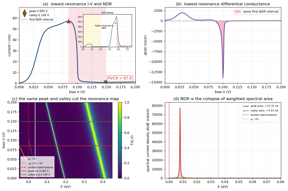
Figure 12. Every main panel refers to the same lowest-resonance cycle. The first current peak is at $0.085\ \mathrm{V}$ and the following valley at $0.149\ \mathrm{V}$; this is the highlighted first NDR interval. The full-sweep inset also shows later, higher-resonance structure near the broader $0.4\ \mathrm{V}$ region, but it is not used to define the first-cycle PVCR.

The quantitative values are

\[I_{\mathrm{peak}}=57.3122\ \mathrm{nA}, \qquad I_{\mathrm{valley}}=0.6519\ \mathrm{nA},\]

and

\[\mathrm{PVCR} =\frac{I_{\mathrm{peak}}}{I_{\mathrm{valley}}} =87.92.\]

These numbers do not come from reading pixels off the transmission map. The heatmap uses a deliberately coarser mesh because it is a visualization of ridge motion.

The quantitative current uses $dE=0.05\ \mathrm{meV}$ and supplements the voltage sweep with $1\ \mathrm{mV}$ spacing around the first cycle. At every voltage the device ramp, collector band reference, and collector chemical potential are rebuilt together:

dE = 5.0e-5                              # eV = 0.05 meV
E_current = np.arange(0.0, E_max + 0.5*dE, dE)
V_current = np.unique(np.round(
    np.r_[V_coarse, np.arange(0.04, 0.2001, 0.001)], 12
))
current = np.empty(V_current.size)

for iV, V in enumerate(V_current):
    U_V = U0 + electron_potential_ramp_eV(N, V)
    T_E = np.fromiter(
        (transmission_fast(E, N, t0, U_V, eps_L, eps_L - V)
         for E in E_current),
        dtype=float, count=E_current.size,
    )
    f_diff = fermi(E_current, E_F, kT) - fermi(E_current, E_F - V, kT)
    current[iV] = current_prefactor_A_per_eV * np.trapezoid(
        T_E * f_diff, E_current
    )

Separating a plotting grid from an integration grid is important. A smooth-looking color map is not evidence that the area under a very narrow resonance has converged. The notebook additionally differentiates the converged current array and uses peak prominence to reject tiny numerical ripples before assigning the first peak and following valley.

Panel (d) uses the same absolute $dI/dE$ scale for peak and valley. The green valley curve is almost invisible because its integrated area is genuinely much smaller; it has not been independently normalized to look comparable.

This is one transparent NDR mechanism in an imposed-ramp one-dimensional model. It should not be advertised as the universal microscopic explanation of every resonant-tunneling diode. Real devices may require charge redistribution, self-consistent electrostatics, scattering, transverse modes, contact nonparabolicity, and hysteretic effects.

---

10. Numerical checks are part of the derivation

NEGF formulas are compact enough that a code cell may run while implementing the wrong physics. The notebook therefore treats identities and limiting cases as part of the calculation, not as optional decoration.

The principal checks are:

• Closed-chain spectrum: analytic and diagonalized eigenvalues agree to $1.33\times10^{-15}\ \mathrm{eV}$.
• Closed eigenstates: $\lVert H\psi_n-E_n\psi_n\rVert<5.5\times10^{-16}\ \mathrm{eV}$.
• Exact elimination: the Schur-complement and projected full inverse agree to $3.48\times10^{-15}\ \mathrm{eV}^{-1}$.
• Surface recursion: the quadratic residual is $2.22\times10^{-16}$.
• Retarded branch: $\operatorname{Im}g_s^R<0$, the $q$ landmarks are $1,i,-1$, and the outside-band branch decays.
• Matched wire: $T(E)=1$ inside the propagating band.
• Single-barrier state: $\operatorname{Tr}(\Gamma_RA_L)$, endpoint transmission, and bond flux agree.
• Spectral identity: the finite-$\eta$ $2\eta G^RG^A$ term closes the equality to $1.77\times10^{-16}$ relative error.
• Equilibrium: $G^n=f(A_L+A_R)$ to $7.26\times10^{-17}$ relative error in the contact continuum.
• Terminal current: the terminal expression reduces to the Landauer integrand to $1.67\times10^{-16}$ relative error.
• Example A: bond current is nearly spatially constant, with the quoted finite-$\eta$ spread, and agrees with the independent Landauer integral.
• Fast solver: the $O(N)$ endpoint calculation agrees with the dense trace.
• NDR quadrature: the plotted peak and valley $dI/dE$ areas reproduce the quoted currents.

These checks diagnose different mistakes. A matched-wire failure points to contact matching or signs. A Schur failure points to block order or conjugation. A current-continuity failure points to $G^n$ indices, bond orientation, energy resolution, or double-counted spin. One scalar “the code ran” test cannot replace them.

---

11. Where this toy model ends

The derivation is exact within its model, but the model is deliberately restricted.

• It is a one-particle, mean-field-like description with no explicit electron-electron or electron-phonon self-energy.
• Transport is phase coherent and elastic.
• The leads are uniform, single-channel, and semi-infinite.
• The effective mass is constant and the grid is one-dimensional.
• Spin enters only as a factor of two; there is no spin-orbit coupling or magnetic structure.
• Example B imposes a linear potential-energy drop rather than solving NEGF and Poisson self-consistently.
• A true bound state disconnected from all continua needs an additional preparation or relaxation model to determine its occupation.

The framework itself extends far beyond these assumptions. Multi-orbital devices replace scalar endpoint quantities by matrices. Additional scattering mechanisms enter through further retarded and in-scattering self-energies. Self-consistent electrostatics updates $H_D$ from the density computed with $G^n$.

The conceptual spine, however, remains the same:

retarded self-energies define the open spectrum and escape;
in-scattering self-energies define how that spectrum is occupied;
Green's functions propagate both pieces through the finite device.

That is the real payoff of the exercise. NEGF is not a bag of unrelated formulas. It is a disciplined way to keep boundary conditions, spectral availability, reservoir population, and conserved flow separate until the final observable is formed.

---

12. Reproduce the calculation

The full executable derivation, including all figures and numerical checks, is available in both locations:

• Run the notebook on Kaggle
• Read or download the source notebook on GitHub

The best reading order is to keep this article open for the derivation and run the notebook section by section for the numerical evidence.

In particular, change one ingredient at a time: the grid spacing, barrier shape, interface hopping, reservoir chemical potentials, or bias profile. The checks above make it much easier to tell a new physical effect from a broken convention.