RSNA Knee, Part 3: Supervision and Public Performance

Select a figure to enlarge it. On small screens, wide tables and equations scroll horizontally.
Recent comparisons do not support a single, reliable ordering of my models. In early October, changing the training labels made local scores worse and leaderboard scores better across five matched imaging setups. Changing only the training objective improved both scores in another experiment. A third comparison kept the labels fixed, changed the image recipe, and again reversed the local ordering on Public. Averaging the scores would hide these differences. I need to distinguish what each experiment changed before deciding what to train next.
Most of the 4,407 training studies have radiology reports rather than the expert annotations used for competition evaluation. A report reader converts the text into twelve target values. Several parts of that process may limit performance: how a finding is defined, what a report omits, which parts of the MRI the model sees, and how its aggregation head combines those images. The strongest public recipes change several of these together. I have to choose which complete systems to reproduce and which narrower hypotheses I can test with the models already available.
N-mm12’s Public result is still unknown. R949F has completed its first fold, but its five-fold reproduction and Public comparison are unfinished. S6F is in code and data preparation. Those results will help determine the next allocation of training and inference time; the experiments below explain why I am pursuing these particular comparisons.
Training targets and the optimal prediction function
For one finding, let $X$ denote the MRI, $R$ its report, $Y$ the desired expert label, and $q(R)\in[0,1]$ the target extracted from the report. With image prediction $p_\theta(X)=\sigma(z_\theta(X))$, binary cross-entropy is
\[\mathcal L(q,p)=-q\log p-(1-q)\log(1-p), \qquad \frac{\partial\mathcal L}{\partial z}=p-q.\]Part 1 used this gradient to explain why a percentile and a probability give different training signals. The consequence goes beyond the update on one example. An ideal learner minimizing unweighted expected BCE, with sufficient capacity and no other restriction, approaches
\[p^*(x)=\mathbb E[q(R)\mid X=x].\]That is the expected report-derived target conditional on the image. It need not equal $\Pr(Y=1\mid X=x)$, the expert-defined quantity whose ranking matters on test. A mild finding may be visible but absent from the report. A reader may interpret “possible” as uncertainty about presence, another as a severity boundary. More examples can make the model better at reproducing either convention without resolving the difference between them. A calibration difference alone need not change AUC; what matters is whether the two conditional quantities order studies differently.
Target transformations therefore change the learning problem. Hardening $q$ at a threshold $\tau$ asks the learner to estimate $\Pr(q>\tau\mid X=x)$ instead of $\mathbb E[q\mid X=x]$. Replacing $q$ by its percentile makes the desired output depend on the score distribution across the dataset. AUC’s invariance to a monotonic transformation of a finished prediction does not make these training operations equivalent.
Confidence weighting changes another part of the objective. For a nonnegative weight $w$ with positive conditional mean, the ideal weighted-BCE solution is
\[p_w^*(x)=\frac{\mathbb E[wq\mid X=x]}{\mathbb E[w\mid X=x]}.\]This can reduce the influence of unreliable examples, but it can also favor conspicuous findings and conventional report language. The target specifies what to learn; the weight specifies how much each example contributes. Label content, target hardening, and confidence weights therefore need separate comparisons, rather than being treated as interchangeable forms of label cleanup.
The local primary metric averages AUC against the Opus- and GPT-derived report-reference tables; v1 is an older reference. Their binary decoding rules are part of their definitions and are distinct from the soft training targets. Complete five-fold OOF supplies image predictions from models that excluded the evaluated fold. The 58 expert-annotated studies, gold58, provide a smaller expert comparison, but I have already inspected them during many decisions. None of these channels is an untouched universal authority on the test ranking.
Agreement and reversals between local and Public comparisons
The first useful evidence came from holding the imaging setup fixed. By October 6, five earlier GPT-label students had matched counterparts trained on the alternative Raptor table:
| Imaging setup | Public, earlier → alternative labels | Public difference | Local primary difference |
|---|---|---|---|
| 64-slice fusion | 0.920 → 0.932 | +0.012 | −0.0054 |
| 80-slice gated model | 0.935 → 0.939 | +0.004 | −0.0157 |
| 2D window model | 0.899 → 0.903 | +0.004 | −0.0204 |
| ConvNeXt-B gated model | 0.923 → 0.925 | +0.002 | −0.0222 |
| 80-slice fusion | 0.934 → 0.936 | +0.002 | −0.0181 |
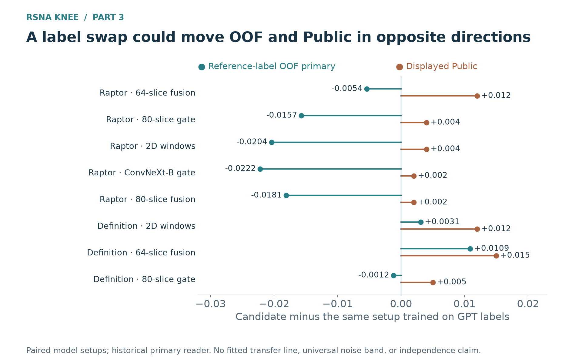 Figure 1. Changing training labels reduced primary and increased displayed Public AUC in five related setups. Shared data and label sources make these related experiments, not five independent estimates of a reversal probability.
These reversals are a reason not to reject the alternative labels simply because primary fell. Shared interpretation between the control’s training labels and local references may explain part of the discrepancy; prevalence, severity encoding, and optimization may also contribute. What I have observed is a reversal. I have not identified a unique cause or a correction factor that translates future local differences into Public AUC.
Giving the report reader explicit finding definitions produced a different pattern. Definition-guided students improved Public by 0.012, 0.015, and 0.005 in three setups, while primary changed by +0.0031, +0.0109, and −0.0012. Removing confidence weights gave a much smaller local change, about +0.0009 with an interval crossing zero. Hardening the definition-guided targets was substantially worse: primary fell by about 0.0147, with negative differences in every fold and all twelve findings. The continuous target encoding was doing useful work in this recipe, even though that result did not tell me whether its useful content was uncertainty, severity, or regularization.
I also needed to distinguish a reference mismatch from a defect in every local comparison. A paired-window DINOv2-B experiment provided a useful counterexample. The two training views had probabilities $p_1,p_2$ and the same study-level target $q$. The control averaged the two losses; the alternative applied BCE after averaging their probabilities:
\[\begin{aligned} \mathcal L_{\mathrm{mean}}&=\frac{\mathcal L(q,p_1)+\mathcal L(q,p_2)}2,\\ \mathcal L_{\mathrm{prob}}&=\mathcal L\!\left(q,\frac{p_1+p_2}{2}\right). \end{aligned}\]At fixed predictions, convexity of BCE in its probability argument gives $\mathcal L_{\mathrm{prob}}\leq\mathcal L_{\mathrm{mean}}$. The distinction matters when a positive study contains windows without the lesion. Mean BCE asks both windows to match the study target individually; probability BCE judges their combined prediction. It better matches the declared probability-averaging inference operation, although the inequality alone cannot establish which trained model will have better AUC.
Here the empirical comparison agreed across channels. With the backbone, labels, input, five-member count, and inference held fixed, probability BCE improved primary by 0.00693, with a recorded paired interval of [0.00534, 0.00859]. Public rose from 0.896 to 0.905. By contrast, the G25 2.5D window model beat the V3 80-slice gated recipe by 0.00942 on primary, with the same definition-label table, but scored 0.929 versus 0.940 on Public.
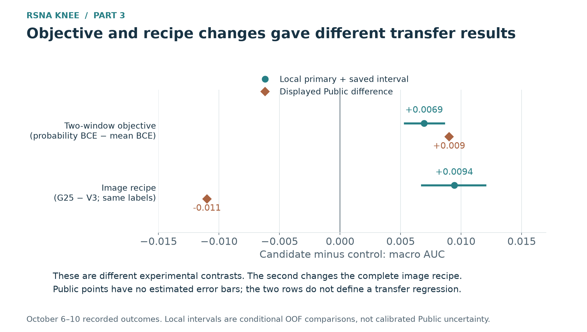 Figure 2. A controlled objective change transferred in the local direction; a whole-image-recipe change with the same labels did not. Local intervals are the saved paired intervals for fixed OOF predictions and references. Public points are displayed outcomes, without an assumed noise model. The two contrasts do not isolate a general architecture effect.
Keeping the labels fixed does not make every local ordering hold on Public. Keeping the architecture fixed helps interpret a label intervention, but does not make the references independent of the target content. I am using local evidence within the scope of each comparison and keeping complete OOF for ensemble analysis. A limited number of declared Public comparisons can then check whether the proposed changes improve test performance. Discarding OOF merely because architectures differ would lose potentially complementary predictions; treating every local ordering as the test ranking would repeat my G25 mistake.
Public recipes: components and reproduction hypotheses
High-scoring public code presents several distinct choices. I can use the published model as a final-only predictor, or retrain its system on my folds to obtain new image-held-out predictions. I can also borrow its crop, attention head, or labels for a narrower experiment. That last option tests a component in another system; it does not reproduce the original recipe. The costs and the comparisons differ for each choice.
The r949 recipe made this distinction concrete. Its 0.949 result combined a CoAtNet encoder, a particular physical crop, per-finding attention, mixed report labels, partially labeled external knees, and mirrored inference. The accompanying performance ladder changed several choices together. It was evidence that the complete system was strong, rather than a measured gain attributable to any single component.
Even the meaning of its input required reading the implementation. Its processed field was a 140 mm centered square resized to 384 pixels; accuracy inference took a 320-pixel center crop, approximately 116.7 mm when the physical crop was not clamped by the source image. This was broader training context relative to its inference crop, not an uncropped whole-DICOM image. Reusing a different 336-pixel cache or the existing head from the 96-slice G96 model would change the hypothesis before training began.
| Recipe | Input and aggregation mechanism | What a new reproduction would test |
|---|---|---|
| r949-derived R949F | Fixed sequence slots; three-slice windows; plain per-finding window attention; mirrored read | Whether the coupled source geometry, training and supervision transfer to declared folds |
| S6-derived S6F | External knee locations; per-finding spatial attention followed by window attention; view and position information | Whether localization and two-stage selection preserve useful evidence more effectively |
| Native-field N | Broad context plus 100 mm local views at field center and physical offsets | Whether retaining context without the same anchor helps alongside a local view |
The aggregation mechanisms differ in what they select. Window attention weights image summaries for each finding. S6 also selects spatial locations inside a window before combining windows, so meniscus and effusion representations can emphasize different regions. Localization can concentrate resolution near the anatomy, but depends on the location estimate and its coverage. N uses a broad context view alongside local views to reduce that dependence. Its declared native reader samples at 0.4 mm up to a 204.8 mm field, retaining aspect ratio and padding the context; “native field” does not mean unlimited coverage at arbitrary resolution.
Training details could alter these mechanisms even when model names matched. The r949 source used one physical study per batch with gradient accumulation over sixteen studies. That does not reproduce the batch-normalization behavior of a physical batch of sixteen. Its external OAI cohort contained 2,399 knees, with only three supervised findings. Masked BCE divided by all twelve target cells, so a partially observed external row did not receive the same normalization as one with twelve observed targets. The external OA and synovitis definitions also differed from my earlier mapping. “Add OAI” was not a sufficiently precise intervention to explain or reproduce its result.
Its supervision had similarly coupled ancestry. Writing $G$ for one Gemini report table, $V$ for a public blended table, and $H$ for the JEV hybrid, the ordinary branch mixed $B=(G+V)/2$ and then $Q=(B+H)/2$. JEV itself used $H=0.95S+0.05E$, where $S$ selected existing public columns and $E$ combined related report reads. Thus, when those sources were present,
\[Q=0.25G+0.25V+0.475S+0.025E.\]An “unstated” branch in $V$ was handled separately. The formula mattered because a newly named table was largely a rearrangement of existing label sources, not a new independent annotator. Source selection and some blending had used exposed expert cases. Retraining image models on held-out folds could protect image-level evaluation, but could not make those reused cases an independent test of the label design.
I am pursuing the complete recipes rather than inferring their performance from component substitutions. R949F has completed its first fold and a small source-input replay; the remaining folds and its Public comparison are still unfinished. S6F uses an ImageNet-pretrained ConvNeXt-S and SKM-TEA V-Net-derived locations, and I have started its port and data preparation. The public S6 route reports 0.950 for an all-data model and 0.948 for a folds-1–4 model, but includes an r949 fallback for unreadable studies. Those scores do not establish how my standalone five-fold reproduction will behave.
This is a substantial allocation of work. The S6F plan estimates 250–310 GB of cache, 10–14 hours of porting, and roughly 9 GPU-hours for five folds, with a pessimistic training estimate of sixteen hours. A stride-one T4×2 read is estimated at 2.9–3.2 hours. These are preparation estimates, not completed measurements. R949’s one-checkpoint 94-window mirrored inference becomes 940 backbone windows per study when all five folds are used. Its strong public result gives me a reason to invest, but I still have to pay for the cache, complete OOF and inference capacity.
Image-assisted supervision and student comparisons
Reports can omit visible evidence. A multimodal reader can instead produce $q(R,I)$ from the report $R$ and a selected image summary $I$. The reader’s apparent confidence is not the criterion I need. I want to know whether an image student trained on those targets ranks studies better.
The pilot used 100 studies outside gold58, each with twelve images: four slices from each of three planes in fluid-sensitive sequences. I compared report-plus-image answers with report-only answers. On 25 studies, I repeated the same input and substituted another study’s images. For effusion, mean absolute probability changes were 0.072 after adding images, 0.014 on repetition, and 0.094 with wrong-study images. Synovitis gave 0.038, 0.016, and 0.040; contusion gave 0.016, 0.003, and 0.043.
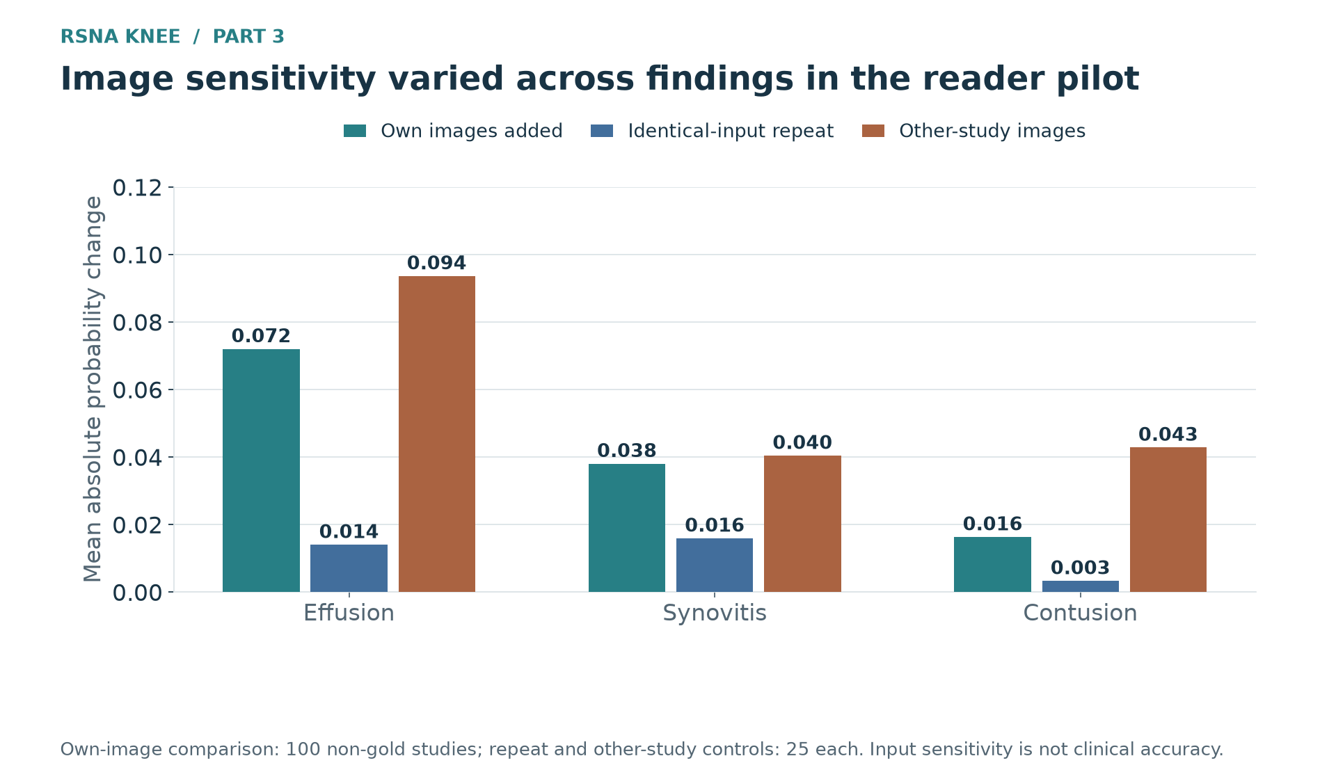 Figure 3. The pilot measured response to image content and repetition, not clinical accuracy. Image addition used 100 studies; repeat and wrong-study controls used 25. Sparse image summaries affected different findings differently.
The stronger response for effusion made an effusion-only update plausible. The other findings created a competing possibility: smaller changes spread across the remaining targets might be more useful than the pilot’s most conspicuous effect. I specified both student comparisons before expanding labeling. mmE changed only effusion; mm12 used the image-assisted targets for all twelve findings. Confidence weights, supervision masks, and the gold rows remained unchanged, making this a target-content comparison rather than a change in which examples counted. The saved usage implied a pilot-plus-corpus estimate near $94.9, not a reconciled invoice.
| Same small 2D student | Primary difference from definition labels | Recorded paired interval | Public |
|---|---|---|---|
| Definition control | — | — | 0.911 |
| mmE, effusion only | +0.0003 | [−0.0029, +0.0036] | 0.912 |
| mm12, all twelve targets | +0.0063 | [+0.0031, +0.0093] | 0.914 |
The all-target version was the more useful result in this student. Its largest primary gains were in lateral meniscus, synovitis, and fracture, rather than effusion alone, while several other targets fell. Sensitivity of the reader’s effusion answer had not identified the best scope of the training intervention. Nor had the wrong-image control established correctness: a fluent reader could be influenced by irrelevant images, and twelve slices could miss a focal lesion. The students tested the value of the resulting supervision, not the clinical accuracy of every changed label.
Stronger learners then tested whether that benefit depended on the visual model. mm12 improved primary by about 0.0064 in the 64-slice fusion student and 0.0037 in the 2.5D window student. More than half the fusion model’s gain came from one fold, making the distribution of the improvement important alongside its pooled value. For a separate 80-slice comparison, I have only verified the first-fold result so far. It does not yet supply another complete five-fold comparison.
The N comparison is an important next result. Its definition-guided version has completed five folds and scored 0.942 on Public on October 14, against 0.929 for G25 with the same definition labels. That difference concerns the complete image recipes, not field of view alone. N-mm12 has primary 0.8913 versus 0.8885, with a saved difference of +0.0027, interval [+0.0010, +0.0044], and positive differences in all five folds. The displayed scores and their difference are rounded separately. I do not yet know its Public result. This comparison holds N’s image recipe fixed, so it can check the new supervision in a stronger learner without assuming that the small student’s gain generalizes.
Teacher content and prior-shrinkage controls
A visual teacher offers another way to connect studies whose reports use different wording. But replacing a report target with a report–teacher mixture changes both its content and its numerical distribution. Improvement after distillation does not identify which part helped.
The first teacher experiment kept the small 2D student fixed. Let $q$ be its definition-guided target, $t(X)$ a teacher prediction, and $\pi$ the target prevalence computed on the training partition. I compared
\[q^{S_b}=0.5q+0.5t(X), \qquad q^R=0.5q+0.5\pi.\]S-b used teacher mixtures for all twelve targets. R pulled targets toward an image-independent prior with the same mixing coefficient. S-a applied the teacher mixture only to effusion, contusion, fracture, and Baker’s cyst. That four-target choice was informed by gold58, so its subsequent expert comparison was exposed.
R was a useful control because it separated a particular kind of prior shrinkage from image-dependent teacher content. It was not an exact match for target entropy: equal coefficients do not make the two target distributions equally soft. The result was nevertheless informative. Relative to the definition control, S-b increased primary by 0.0078, while R decreased it by 0.0092. Directly comparing S-b with R gave +0.0170, with a recorded interval [+0.0141, +0.0200], positive in all five folds and all twelve findings.
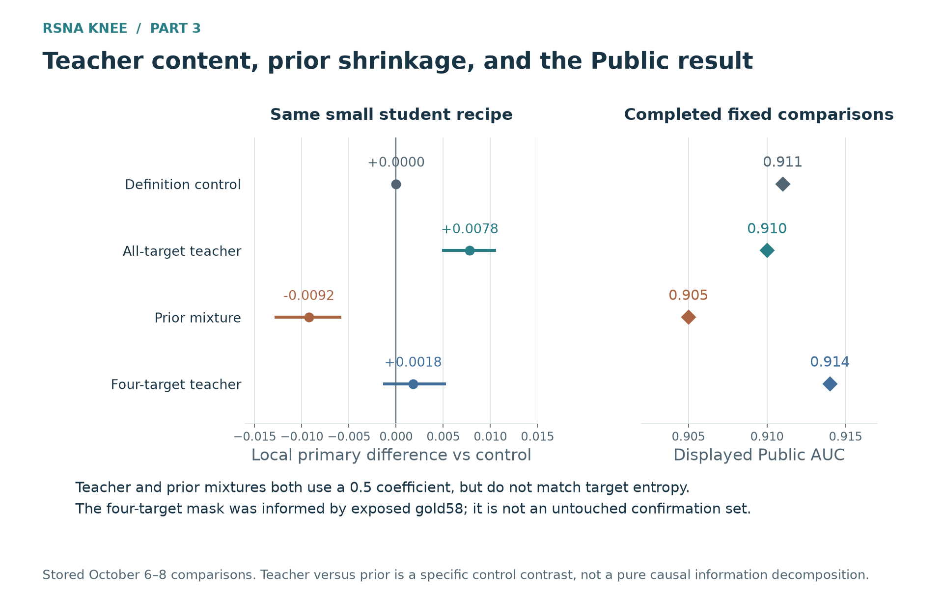 Figure 4. The same student under definition targets, all-target teacher mixtures, a prior mixture, and a four-target teacher mixture. Local intervals describe paired differences on the stored OOF predictions. The four-target mask used exposed gold58; the Public outcomes are transfer evidence rather than an independent validation of that mask’s selection procedure.
Public added an important qualification. S-b scored 0.910, R 0.905, and S-a 0.914, against the control’s 0.911. Teacher content beat this prior control on Public as well as primary, but the all-target teacher still failed to beat the original control’s displayed score. The local winner was S-b; the Public winner was S-a. The reused expert panel had favored the prior mixture, which finished lowest on Public. Choosing any one channel as the general ranking authority would have missed another part of this experiment.
I am continuing to investigate teacher content without treating all-target distillation as universally better. An image-dependent teacher may recover information beyond the report, but its strength, target coverage, and interaction with the student matter. Rather than multiply variants of the same weak teacher, I also ran comparisons with a stronger teacher mixture.
Stronger teachers and evaluation-fold exclusions
For nonnegative weights summing to one, BCE is linear in its target:
\[\mathcal L\!\left(\sum_s\lambda_s q_s,p\right) =\sum_s\lambda_s\mathcal L(q_s,p).\]A supervision mixture is therefore an explicit weighted compromise among the sources’ learning instructions. This identity does not make separately trained students equivalent to one student trained on mixed targets. It does make clear what the stronger T* recipe asked a student to learn:
\[q^{T^*}=0.50\,q^{\mathrm{definition}} +0.25\,p^{\mathrm{ensemble}} +0.25\,p^{\mathrm{public\ S6}}.\]The public visual teacher may add distinctions missing from report interpretation. Its training history also raises an evaluation problem. For a student holding out fold $j$, consider a training example in fold $k$. A teacher excluding only $k$ may have learned from $j$. The student’s training targets can then contain information from its validation labels even though it never trains directly on the validation images.
Protecting the student evaluation requires excluding $j$ from teacher training. The B2 construction used in the earlier controlled experiment additionally excludes $k$, keeping the training example’s teacher target itself out of sample. The available T* ensemble and public predictions do not establish the required exclusion of the student’s evaluation fold. T* students and their descendants are therefore final-only: usable for test prediction, but excluded from clean-OOF ensemble selection. Training the student locally does not remove information inherited through its teacher.
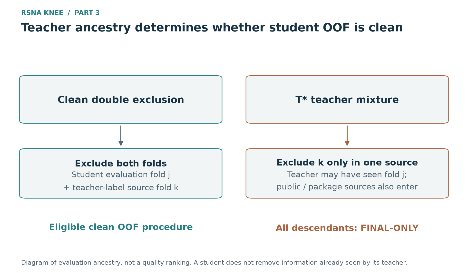 Figure 5. B2 excludes both the student’s validation fold and the source example’s fold. T* uses stronger available predictions without that guarantee. This teacher-training issue is separate from exposure of expert cases during report-label design.
The G25 T* student scored 0.945 on October 14, against 0.939 for its earlier ensemble-teacher version and 0.929 for definition-guided supervision. This morning, October 15, a G96 T* student also scored 0.945, compared with 0.934 for its earlier no-OAI Raptor-label version. The G96 change also used definition-derived ranking pairs and label-aware batches, so it compares supervision recipes rather than an isolated target-mixture coefficient. Both students inherit overlapping teacher sources; these scores are not two independent discoveries of new visual information.
These results support further work on stronger visual supervision, but the optimistic local values remain unsuitable for clean-ensemble selection. A comparison against a B2 teacher would change teacher content and training construction together; it would not isolate the effect of leakage. I am preserving clean image-held-out families for conditional ensemble analysis and evaluating final-only students through declared external comparisons, with their teacher ancestry recorded.
The next decisions depend on three comparisons. N-mm12’s Public result is still unknown. R949F and S6F need complete reproduction and runtime evidence before I can judge whether their improvement justifies the preparation and inference cost. Stronger teacher-derived students also need to be compared alongside the image models: they may complement them, or mostly repeat rankings inherited from shared teachers. I will allocate the next training and inference time using those results. No single report reader, reused expert panel, or Public point can settle all three comparisons.