RSNA Knee, Part 5: Model Building in a Changing Competition

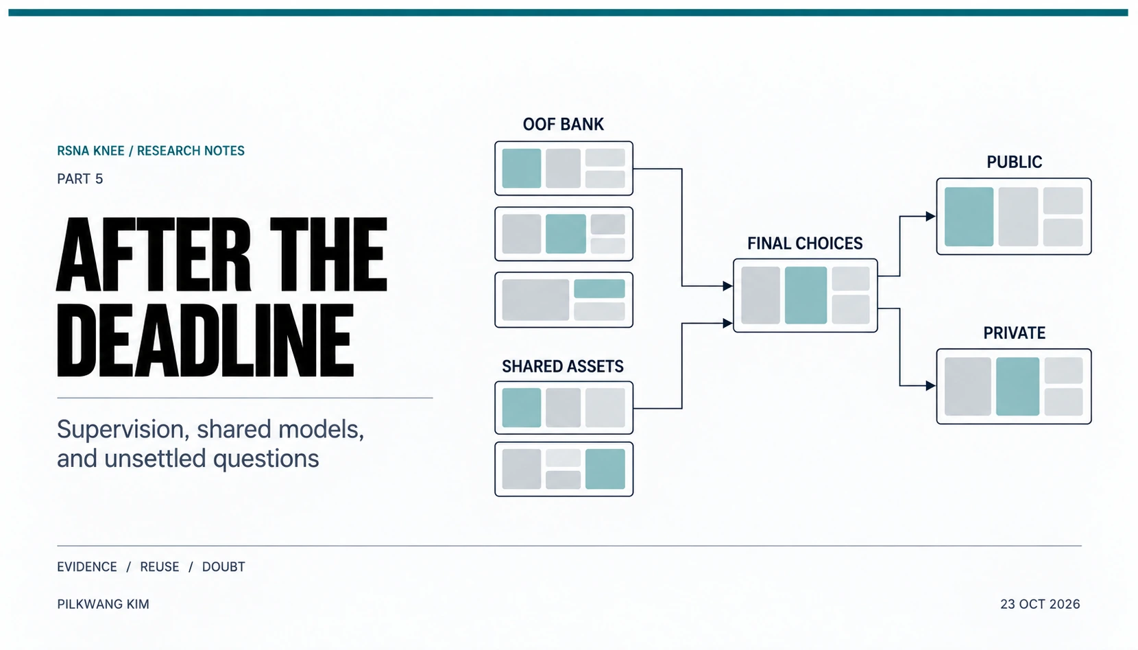
Select a figure to enlarge it. On small screens, wide tables and equations scroll horizontally.

In this final part

Competing solo, I finished 560th out of 6,425 teams, with a Bronze Medal. This final article follows the development through the standings and 154 paired submission scores: which model and supervision changes improved Private, and why the late extensions did not take the results further. The public H system remained stronger than my best completed clean composition. Adding my predictions improved the final H mixture, but that small contribution left the weakness of my own system unresolved. I revisit the OOF investment, the role of supervision and public releases, and the frustration of spending so much time on a result I had wanted to be stronger.

---

Final result

My final Private AUC was 0.943. Of the two submissions I selected, the H-dominated rank blend, v229, determined that score. The clean S6F-heavy composition, v236, scored 0.941. Looking across all my scored submissions after the reveal, v229 also had the highest displayed Private score.

Candidate	Public	Private
H alone, v219; my Public best	0.958	0.942
H + 25% own rank block, v229; selected	0.957	0.943
K-W2, v236; selected	0.953	0.941

My position in the official standings moved from Public 1,785th to Private 560th, a rise of 1,225 places. This rank change and v229’s 0.957 → 0.943 describe different comparisons. My Public best was H at 0.958, whereas my final Private result came from v229. The two leaderboard scores need not belong to the same submission. In the submission-level analysis below, I avoid that ambiguity by pairing the scores of each exact submission.

I retrieved the official leaderboard and my submission history on October 23. The account returned 177 attempts, of which 154 had both scores. One of those was a known deployment failure that scored 0.500 on both splits; I separate it from the 153 model-performance observations. The other 23 attempts had no paired numerical result. All values here retain Kaggle’s three-decimal display precision. A displayed tie is not proof of identical predictions or exactly equal AUC.

Public–Private rank changes

Private was lower than Public for much of the board. Across all 6,425 matched teams, the median difference, Private minus Public, was −0.016, with the middle half between −0.018 and −0.015. My leaderboard score difference of −0.015 was therefore close to the middle of the observed distribution. The drop was not unusual by itself.

The Public leaders nevertheless remained broadly competitive. Public winner Barry moved from 0.970 to 0.957 and finished 7th. Private winner Team Kangaroo moved from Public 4th, 0.969, to 1st, 0.960. Seven of the Public top ten remained in the Private top ten.

Public cohort	Also in the same Private top group
Top 10	7 of 10
Top 100	84 of 100
Top 500	418 of 500

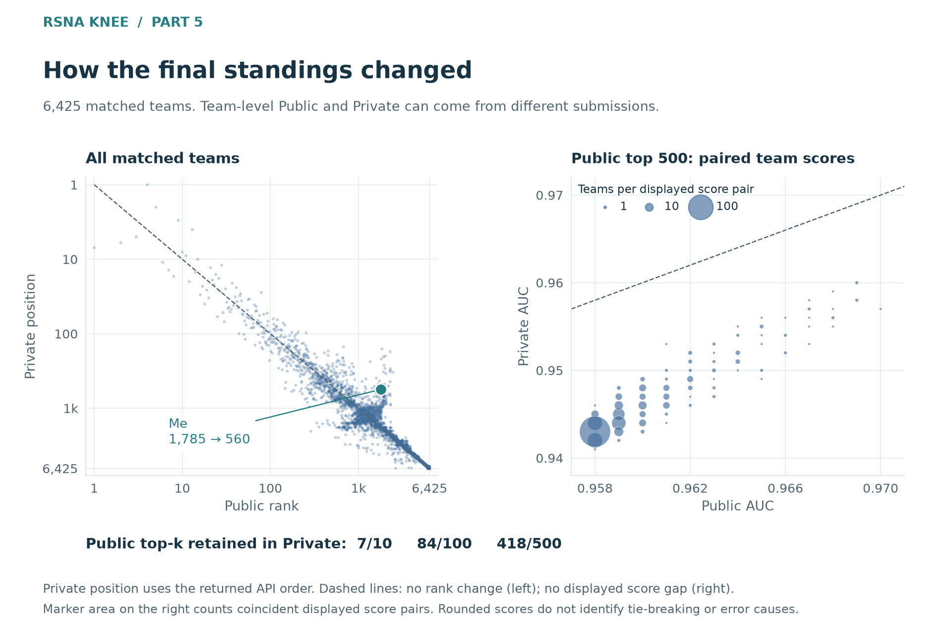
Figure 1. Official Public ranks are joined to the complete ordered Private leaderboard by team ID. The diagonal marks no change. The score panel uses the Public top 500; I am outside that cohort, so my result is marked only in the rank panel. Team Public best and final Private may come from different submissions.

The large 0.958 Public block was especially important to my finish. By the final snapshot it contained 1,638 teams, occupying Public ranks 257–1,894. Of those teams, 1,239 finished at a displayed Private score of 0.942. The block’s Private scores nevertheless ranged from 0.899 to 0.946, and its Private positions from 150th to 4,197th. A common rounded Public score was plainly not enough to identify the final prediction.

This density helps explain why a small score advantage could accompany a large rank gain. My v229 finished at 0.943, just above the block’s most frequent Private display of 0.942. That does not explain every place gained, or establish that every team in the block ran a copied notebook. It does show why “I moved up more than a thousand places” and “the score advantage was small” can both be true. The broad ordering remained informative; fine distinctions among closely packed candidates were much less secure.

Development and score progression

The full history shows improvement on both splits. The first frozen-encoder baseline scored 0.711 / 0.680 on Public / Private, and the selected final submission scored 0.957 / 0.943. Those are increases of 0.246 and 0.263, respectively. Many parts of the system changed between these endpoints, so the differences describe the development as a whole rather than the effect of any one method.

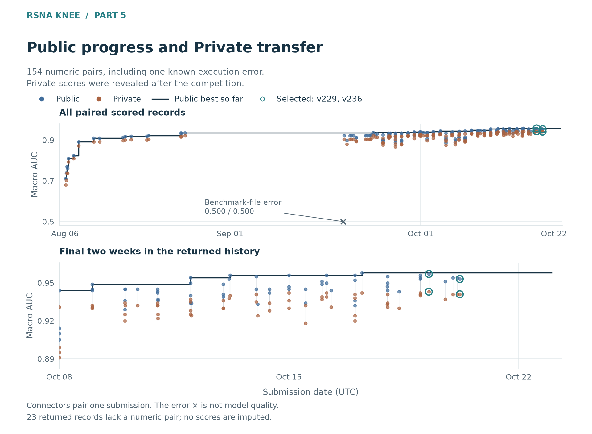
Figure 2. Scores are placed at their actual submission timestamps. Private values were revealed after the deadline and are shown retrospectively. The Public-record sequence is descriptive, not a claim that I knew its Private values during development. Unscored attempts are not assigned zero AUC; the known 0.500 deployment failure is identified separately.

Submitted, UTC	Main change or candidate	Public	Private
Aug 6	Frozen DINOv2-S baseline	0.711	0.680
Aug 8	Fine-tuned, four-seed DINOv2-S ensemble	0.891	0.871
Aug 19	Expanded own package and auxiliary arm	0.921	0.904
Aug 24	Public CoAtNet blended with the own package	0.935	0.921
Sep 30	Compact V3 + DK rank blend, v84	0.940	0.928
Oct 11	Updated own-family package, v161	0.945	0.934
Oct 12	Public R949 + S6 pair, v170	0.954	0.937
Oct 15	Native N with mm12 targets, v201	0.945	0.932
Oct 16	Native N with T* teacher targets, v203	0.951	0.939
Oct 17	Five-fold S6F reproduction, v213	0.952	0.938
Oct 17	Public H recipe, v219	0.958	0.942
Oct 19	S6F + N + V3, K-W v231	0.954	0.941
Oct 19	H + 25% own rank block, v229	0.957	0.943
Oct 20	Second S6F seed, K-W2 v236	0.953	0.941

This is a set of milestones and controlled-comparison candidates, not a monotonically improving sequence. Dates are UTC. The complete paired history is available as CSV.

The early gains came from making the images and the supervision usable: fine-tuning the encoder, fixing the input geometry, improving slice coverage, and combining completed families. By August 19, Private had reached 0.904. Later compact own-family packages reached 0.928 and then 0.934. The public systems raised the available test predictor further, but they were not the only source of progress.

A short guide to the recurring model names

• N: the native-field 2.5D ConvNeXt-S learner, combining wider context with local views.
• V3: the 80-slice image model used in the compact own block.
• S6F: the public S6 recipe reproduced on my folds, with ConvNeXt-S and finding-specific spatial/window attention. A reproduced recipe is different from directly using public weights.
• H: the public blend of R949, R224 and R6-flip predictions.
• mm12: targets for all twelve findings constructed with reports and selected images.
• T*: targets combining definition-guided labels with stronger teacher predictions; the resulting students are final-only.

The final fortnight followed several branches at once. An individual N model, a teacher student, an S6F reproduction and a public mixture tested different hypotheses. They were not successive additions to one fixed ensemble. The question was how to use the information in those families to obtain a prediction worth the cost of executing it.

Training targets and Private performance

The most useful comparisons hold a learner’s declared recipe fixed while changing its targets. In the native N engine, replacing definition-guided targets with mm12 moved Private from 0.928 to 0.932, alongside a Public gain from 0.942 to 0.945. Replacing mm12 with blendjev moved both scores down by 0.002. The label table that worked well in one recipe was not automatically better in another.

Stronger teacher targets produced larger changes. N-mm12 → N-T* increased Private by 0.007; G25’s definition-target student → G25-T* increased it by 0.014. These are observed Private improvements of the submitted systems. They do not qualify the students for clean-OOF combination selection: the T* teacher content did not establish the necessary fold exclusions. Shared teacher content is also a reason not to count these students as independent sources of new information.

Submitted comparison	Δ Public	Δ Private
N: definition targets → mm12	+0.003	+0.004
N: mm12 → blendjev	−0.002	−0.002
N: mm12 → T* teacher targets	+0.006	+0.007
G25: definition targets → T*	+0.016	+0.014
R949F → S6F recipe	+0.008	+0.007

The label contrasts describe one trained-family pair each. R949F → S6F changes several coupled parts of the system. The table is not a decomposition of independent causal effects.

The original supervision problem remains important even after those scores are available. Most training studies supplied reports rather than complete expert annotations. An explicit negative, an uncertain statement and an unmentioned finding are different observations. A more capable report reader can interpret a statement that is present; it does not directly observe the image finding omitted from the report. The report–label inconsistencies discussed during the competition therefore belonged inside the modeling question.

If the training target is $q\in[0,1]$ and the image is $X$, an unrestricted function minimizing the population loss of unweighted binary cross-entropy has optimum

\[f_q^*(x)=\mathbb E[q\mid X=x].\]

That need not equal the desired image-finding probability. It can still preserve the desired ranking under some forms of missingness, so the equation is not an impossibility result about learning from incomplete reports. The question is whether constructing $q$ preserves the distinctions needed for the image task. Class weighting, sampling and finite model capacity complicate the actual learner further. Changing the optimizer does not answer that question for me.

This gives target construction a role that better optimization alone cannot fill. Fitting an incomplete report target more accurately does not ensure a better ranking of the desired image findings. Multimodal targets and a stronger visual teacher can introduce information absent from the original target. Yet the opposing N results also matter: more information, or a more elaborate labeling procedure, does not guarantee better learning in a particular model.

S6F added another route. Relative to R949F, its Private gain was 0.007. The r949blendjev target table was retained, while the backbone, anatomical input route, attention, training and aggregation changed together. The result supports the complete reproduced system; it does not identify the contribution of any one of those changes. Learning that interaction required more than importing an individual layer into an older pipeline.

Domain knowledge also entered through what counted as a positive finding, which anatomy the input retained, and how credible a report-derived negative was. External labels and anatomical priors could supply information unavailable from another search over the existing bank. The public CoAtNet recipe connected those decisions rather than offering a backbone in isolation. That broader role of supervision is separate from the matched R949F → S6F comparison above, which retained its target table. My specific target-table comparisons show that supervision changed my submitted results. How much external data, outside labels and domain knowledge explain the competition-wide frontier remains a hypothesis to examine against complete public recipes and post-competition write-ups. Those two levels of claim should not be conflated.

Ensemble composition

S6F alone reached 0.938 on Private. Combining it with N and V3 in K-W reached 0.941. The equal-family K-eq composition scored 0.940; increasing S6F’s share to one half gave the extra displayed 0.001. That is a concrete benefit from a clean composition, even though the strongest final candidate also used public predictions.

A different four-family combination, D2c, fell from S6F’s 0.938 to 0.933. Adding the three families also reduced S6F’s weight from one to one quarter, so I cannot divide the loss into an independent negative effect from each added model. The observation belongs to the complete composition. Likewise, expanding a compact earlier package into the broader R1-C proposal reduced Private from 0.931 to 0.923. Completing more families created options, but putting more of them into an ensemble did not always help.

The H comparison is the clearest small reversal between Public and Private. With $R$ denoting a per-finding rank transformation and $A_{10}$ my N/V3 member-rank block, the tested outer operator was

\[C_\alpha=(1-\alpha)R(H)+\alpha R(A_{10}).\]

H alone scored 0.958 / 0.942. With own share 0.25, v229 scored 0.957 / 0.943; with own share 0.50, v227 scored 0.956 / 0.942. Public preferred H alone. Private preferred the tested quarter-share mixture at the displayed precision. My own predictions contributed to the best submitted result, while giving them more weight did not improve it further. The complete H mixtures remained final-only, regardless of the clean identity of their own components.

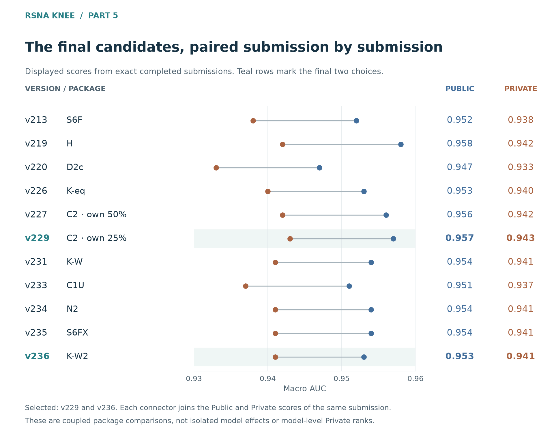
Figure 3. Each row pairs the Public and Private scores of one exact submission. Highlighted rows are the two selected candidates. These are observed AUCs, not confidence intervals; a displayed tie does not establish equal predictions or statistical equivalence.

Late extensions

Several last extensions failed to improve that result. Adding a fourth family in C1U reduced K-W’s Private score from 0.941 to 0.937. It also changed the existing family shares, so the observation cannot be assigned solely to the fourth family’s standalone quality.

The second N seed in N2, a full-data S6F checkpoint in S6FX, and the second clean S6F seed in K-W2 all ended at a displayed Private 0.941, equal to K-W. K-W2’s Public score was lower by 0.001. The clean OOF evidence that motivated its second-seed bag did not become a visible test-score gain in this run. That is a much narrower conclusion than saying bagging is useless, or that the original OOF measurements were false.

The larger candidates expected to exceed the time limit never produced scores. The K-W3 sequence ended with a platform system error, a timeout on retry, and an unhandled error on the final retry. Other expanded reads also had time-limit or execution failures. Without scores, I cannot establish that these models would have been weak or strong enough to change the result. What I do know is that a model unable to complete the declared test execution was unavailable for final selection.

Across the 154 paired numerical outcomes, no displayed Private score exceeded v229’s 0.943. The development process matters more here than reconsidering the last selection alone: why did the completed systems reach this level and stop? The execution failures identify options I lost, but cannot tell me what those options would have scored.

The Public–Private gap

AUC depends on positive–negative pairs within each finding. Changing the held-out studies changes those pairs, and rare findings can be sensitive to which difficult cases appear. Repeated choices informed by Public can also favor that split. In addition, the team-level board compares Public-best submissions with a final selection. These are different mechanisms; one score gap does not tell me their separate contributions.

The broad Public–Private score ordering was strong: Spearman correlation across the 6,425 displayed team-score pairs was 0.986. That is compatible with the final small reversals. A statistic dominated by the board’s broad performance range does not make a 0.001 Public advantage a reliable choice among near neighbors.

My own experiments need the same distinctions. Better supervision and stronger complete recipes often improved both splits; the late fixed-share H comparison favored different choices on the two splits; extra seeds mostly reached displayed ties. These observations do not support a single verdict that Public was either trustworthy or meaningless. Aggregate scores also cannot establish the clinical cause of a gain, measure model-error correlation, or provide a per-study uncertainty interval. Those analyses would require the corresponding test predictions and labels.

My systems and H

The central comparison is straightforward. My completed clean compositions topped out at displayed Public 0.954 and Private 0.941. H alone scored 0.958 / 0.942. The systems I had actually trained, executed and submitted were weaker on both splits. I had hoped that H might be particularly suited to Public, leaving my clean-evidence route an advantage on Private. The result did not support dismissing H as merely Public-overfitted: it remained stronger than my completed clean packages. The amount of complete OOF I had produced could not substitute for that performance comparison.

Adding my own block raised H’s Private result to 0.943. A useful addition to a stronger predictor is nevertheless a different achievement from building a stronger predictor myself. I had achieved the former. This comparison covers completed, scored packages; it does not establish the best possible combination of every file in the bank. Within that scope, my delivered systems still fell short of H.

I did not turn the available data, training time and accumulated evidence into a system of my own that surpassed the public one. The shortfall went beyond the last choice of a model or weight. I had treated too much of the task as a problem to solve with generic ML techniques, more training and a larger bank, without reconsidering the learning problem deeply enough. Choosing what information to obtain, what the targets should mean and which complete system to reproduce was part of modeling too. My framing had left those questions with too little attention.

The size of the final score difference is only known at display precision; it does not identify which decision caused the shortfall. I also cannot establish the counterfactual in which those public notebooks never appeared. My own bank might have occupied a higher relative tier in that setting, but that is an untested hypothesis. The actual competition included those systems, and I had to build something useful in their presence.

The OOF bank

I built complete OOF families because I wanted the research to accumulate. A completed family left predictions on studies excluded from its training. Another family could be compared on the same studies, and a combination rule could be chosen inside the other folds before being evaluated on the held-out fold. A new run could then be judged alongside alternatives, rather than simply added to the last package.

That required more than keeping checkpoints. Fold assignments, study keys, target definitions and aggregation operators had to agree. An incomplete promising run was not interchangeable with a complete family. I accepted the cost because the resulting predictions were supposed to make later choices better, not merely make the archive larger.

The bank made those comparisons possible. It could not guarantee that its families were strong enough, that I had explored the most valuable hypotheses, or that another combination search would overcome the limits of the available predictions. A careful comparison can rank a set of candidates correctly while all of them fall below a stronger system. The quality of my evidence and the strength of my predictions were separate questions.

The late public parents also created a second evaluation problem. Some used all competition training studies; others did not expose enough ancestry to reconstruct compatible exclusions. Teacher content could carry the same issue into a student. My own components retained their clean identities, but adding them could not make the complete public mixture clean.

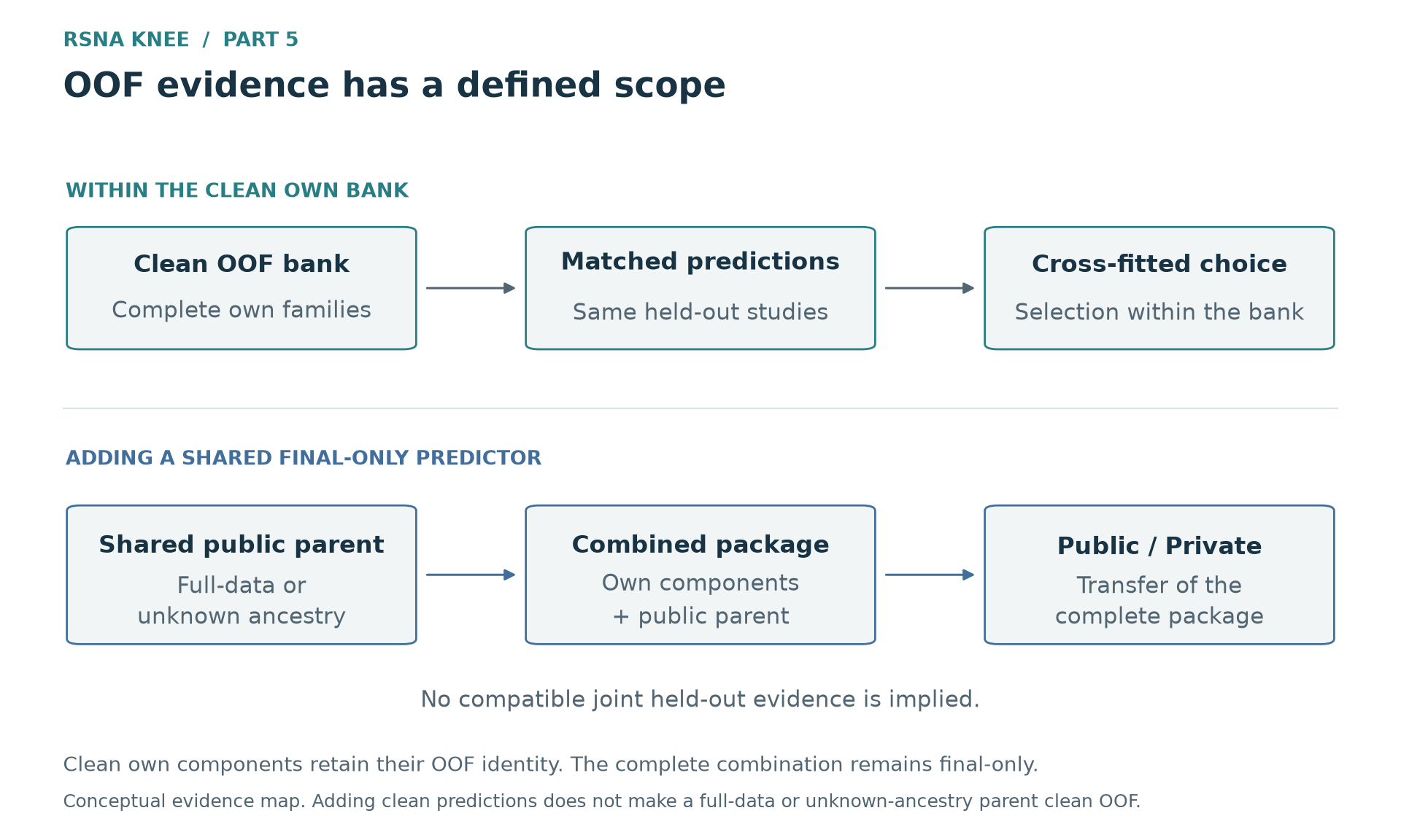Figure 4. Conceptual evidence map. Compatible own-bank predictions support cross-fitted combination selection. A full-data or unknown-ancestry parent needs different evidence for the complete mixture. The diagram contains no measured performance quantities.

The bank therefore remained useful while falling short of the role I had wanted for it. I had invested in those assets to guide the choice of a strong final predictor. At the finish, I mainly used them to find a small improvement to a stronger public system. Those were different outcomes for me. The assets retained their scientific use but had lost much of their relative competitive value.

A shared baseline

A new notebook, a new reducer and a new source of predictive information were not the same event. Some releases supplied a useful training system or genuinely different weights. Others reused much the same content through a different assembly. Deduplicating those lineages mattered because a growing list of notebook names did not imply equally many independent ideas.

Once a strong runnable system became widely available, the standalone quality of my predictor was no longer enough to judge its practical value. Let my predictor be $u$, the shared baseline $b$, and the declared combination operator $C$. For an evaluation metric $M$ on the same held-out studies, the relevant difference was:

\[\Delta M=M\!\left(C(u,b)\right)-M(b).\]

The metric must be the same and the matched evaluation valid. A good standalone $u$ can still add little information that corrects the ordering errors of $b$. A different architecture, substantial training effort and complete OOF give me reasons to test that contribution, but cannot guarantee a gain. By the finish, I was asking what I could add to the stronger shared predictor. The H comparison gave a small observed improvement, though this was far from the central role I had expected my bank to play.

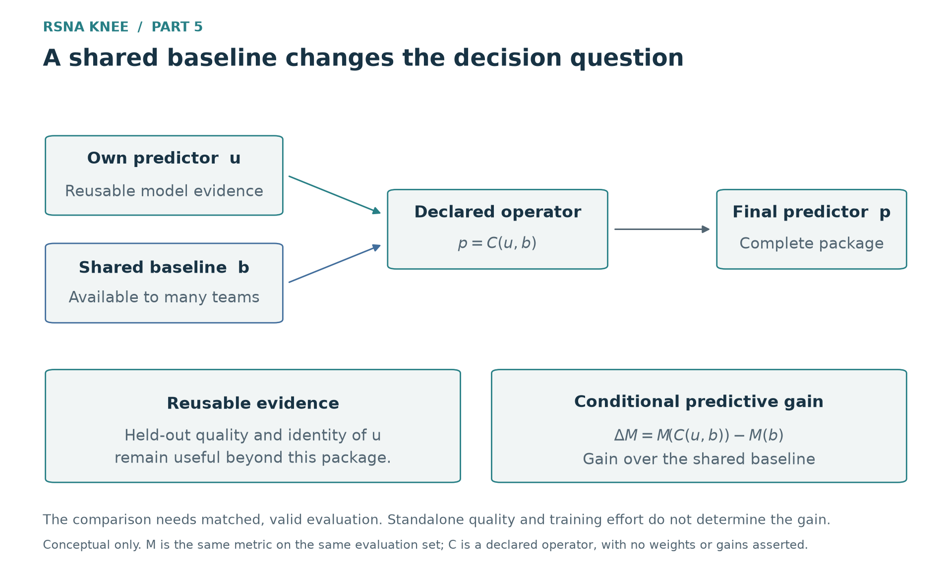Figure 5. Conceptual comparison. The usefulness of an own predictor depends on the parent and the combination operator. The diagram assumes no fitted weight, independence or numerical gain; the actual candidates are measured separately in Figure 3.

Making those systems public did not diminish the research behind them. I benefited from the released readers, labels, training code and predictions, and a rounded leaderboard score told me little about the effort behind anyone else’s work. What I found difficult was the role my own work had come to occupy. I had expected it to provide the main predictor; instead, it became a small component complementing a system I had not matched.

Research priorities and execution costs

Finding a promising method was not the same as having a prediction ready to compare. A label table needed its values interpreted. External data needed compatible target definitions and a route into training. A checkpoint needed its input assumptions and inference implementation understood. Training, complete OOF, export, replay, full-scale execution and collection each consumed time before a result could inform the final choice.

The nine-hour limit made the opportunity cost concrete. A scientifically interesting addition could be too expensive for the final read. A compact, coherent recipe could therefore be more valuable than several individually promising models whose combined execution did not fit. The scoreless expanded candidates are actual consequences of that constraint; they do not tell me what those candidates would have scored with unlimited time.

A comparison I could interpret precisely was not necessarily the experiment I should prioritize. Holding an engine fixed and changing one target table could reveal that difference clearly, without making it worth the next week of work. Some larger changes were harder to isolate but more consequential than another variation within a familiar formulation.

There were two ways to spend the remaining time badly: integrate one release after another without learning what made the system stronger, or insist on a comparison so complete that it could no longer finish before the deadline. Recognizing the difference, preparing the useful alternatives early and bringing them to an interpretable result were part of my responsibility. A process that kept producing files and checks was not enough by itself.

Lingering frustration

Acknowledging the weakness of my completed systems does not remove the frustration. I had invested in complete OOF to build a strong predictor, rather than simply leave an orderly archive. In the final fortnight, carefully prepared models often felt like material to search for a small addition to something stronger.

Effort does not entitle a model to a higher score. The fact that I could reuse the files later did not, however, answer whether this had been a satisfying way to spend the time. The final score evaluates a prediction. It does not evaluate the value of every experiment, the cost of producing the evidence, or whether I want to repeat the process.

Knowing the Private results now can make the earlier choices seem clearer than they were. At the time, I did not know those results, and the scores of unfinished experiments remain unknown. I can describe the shortfall more specifically without finding the experience any less frustrating.

Formula 1 and participation costs

In a Name That LLM discussion about the cost of generating additional training data, participants compared Kaggle to Formula 1: skill still mattered, but so did the resources available to put that skill to work. Others replied that resources had always affected competition and that useful results were still possible on modest budgets. These were participants’ views, not an official explanation of what determines a result. I recognized something of my own experience in the comparison.

I increasingly feel that some competitions reward an entire development operation. Model design is one part; acquiring useful data, preparing inputs, running enough comparisons and getting the complete system to execute are others. Like a driver needing a capable car and the preparation behind it, my ideas needed data, hardware and implementation to become useful predictions. I had underestimated how much of the competition involved doing all of this well.

The late public releases reduced some demands while adding others. Strong systems made sophisticated predictions accessible to more people. Yet each release could bring another round of preparation and comparison before an earlier candidate had even finished evaluation. Easier access did not necessarily mean less work to participate. I was grateful for the open research and exhausted by having to reconsider what to use.

Efficient inference, data preparation and reliable execution are substantial skills. Near the end, though, more of my attention went into keeping up, repeating familiar comparisons and making everything finish on time. I spent longer at the keyboard without a corresponding sense that I understood the problem more deeply. For me, the experience had begun to feel more consuming than instructive.

Accepting my shortcomings does not automatically make me want to enter another competition on the same terms. Being willing to learn how to compete and wanting to devote this much time to competing are separate choices.

Future participation

For now, I plan to take part in tabular competitions only casually. Rather than spend weeks adjusting features, hyperparameters and seeds for a small improvement in rank, I would prefer to read the solutions after the competition ends. A more serious commitment would need a new domain to study or a difficult validation problem I want to work through.