RSNA Knee: Twelve Findings From One MRI, and the Reports That Label Them

RSNA Knee: Twelve Findings From One MRI, and the Reports That Label Them

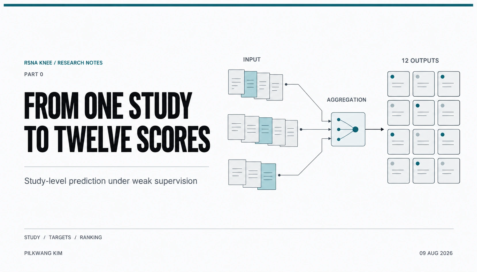
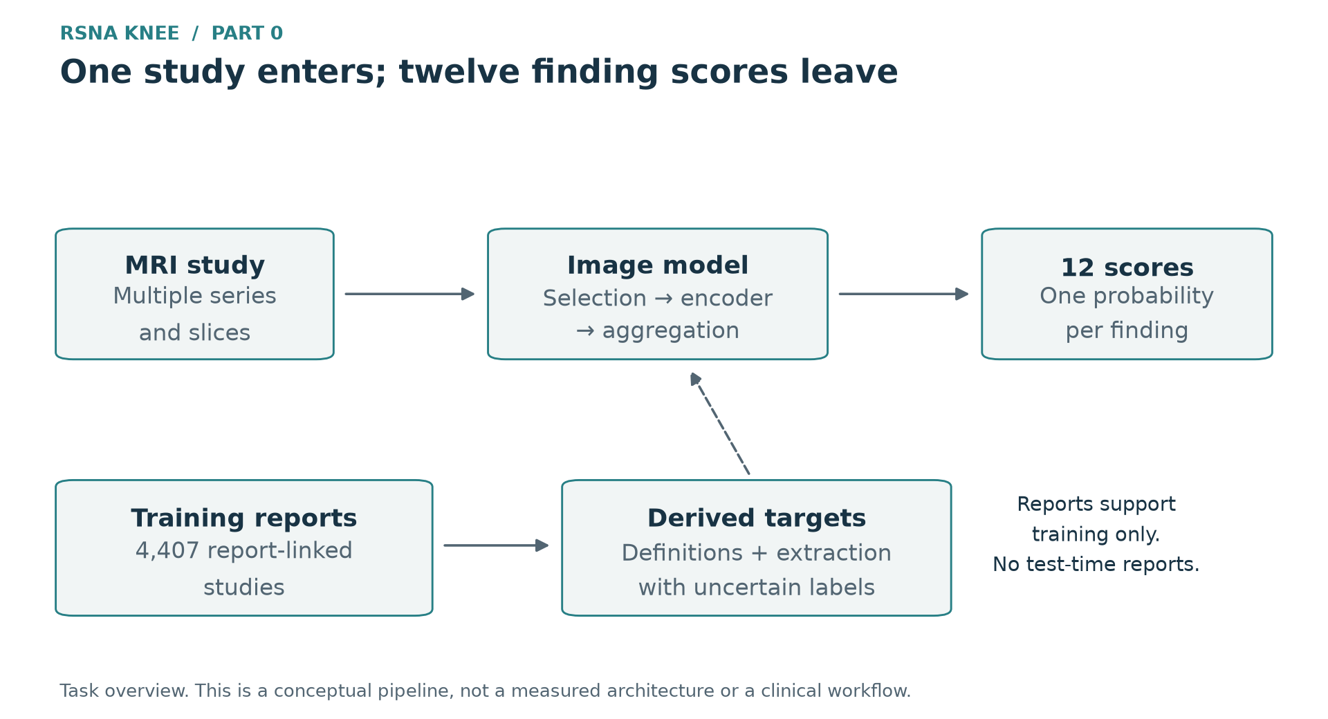
The RSNA Knee Abnormality Detection competition asks for twelve probabilities per MRI study. It looks like a 3D medical imaging problem. It is not, or not only: of 4,407 training studies, 58 carry per-condition annotations and the remaining 4,349 carry a free-text radiology report in one of nine languages. The imaging model is downstream of a text problem that has to be solved first.

This article develops the pipeline in my public notebook from first principles — what the metric permits, what the DICOM headers make recoverable, what the sampling theorem forbids, and where the supervision actually comes from.

Korean version: 주석은 58건, 판독문은 4,407건 — RSNA Knee 대회의 구조

Key links:

• RSNA Knee Abnormality Detection
• Notebook: RSNA Knee baseline v1

---

1. What the metric permits

The score is the unweighted mean of twelve per-label ROC AUCs:

\[\text{Score} \;=\; \frac{1}{12}\sum_{i=0}^{11} \mathrm{AUC}_i .\]

Three consequences follow directly, and each removes a design decision rather than adding one.

Only order matters. $\mathrm{AUC}_i$ is invariant under any strictly increasing map of the scores for label $i$. Calibration is worth nothing and a threshold is worth nothing. It also settles how to combine models: averaging raw probabilities lets whichever model happens to be most confident dominate, whereas averaging ranks combines exactly the information the metric reads. Every combination below is a rank mean.

Every label costs the same. Write $M$ for the mean AUC a good model reaches. A label left at chance contributes $0.5$ instead of roughly $M$, forfeiting

\[\frac{M - 0.5}{12}\]

of the final score however well the other eleven do.

At $M = 0.85$ a single chance-level label costs 0.029 — larger than the gap between neighbouring places on a mature leaderboard. Rare findings therefore deserve more attention than common ones, because a rare finding is where a model most easily ends up at chance.

Prevalence drift is survivable; thresholds are not. AUC is in expectation invariant to the positive rate. The competition states that prevalence is not guaranteed to match across the training, public and final sets — fatal for an accuracy-like metric, harmless here.

---

2. Where the supervision comes from

The decisive structural fact is in the schemas rather than the prose: train.csv has a Report column and test.csv does not. Text is available when fitting and absent when predicting. That rules out any model with a text branch — at inference it would have nothing to read — and leaves three admissible uses of the reports:

1. turn them into training targets, then fit a pure imaging model;
2. use them as an auxiliary training signal, distilled into the encoder and dropped at inference;
3. use them to weight studies by how confidently their labels could be read.

The notebook takes the first and the third.

2.1 Two readers, and how to tell which is better

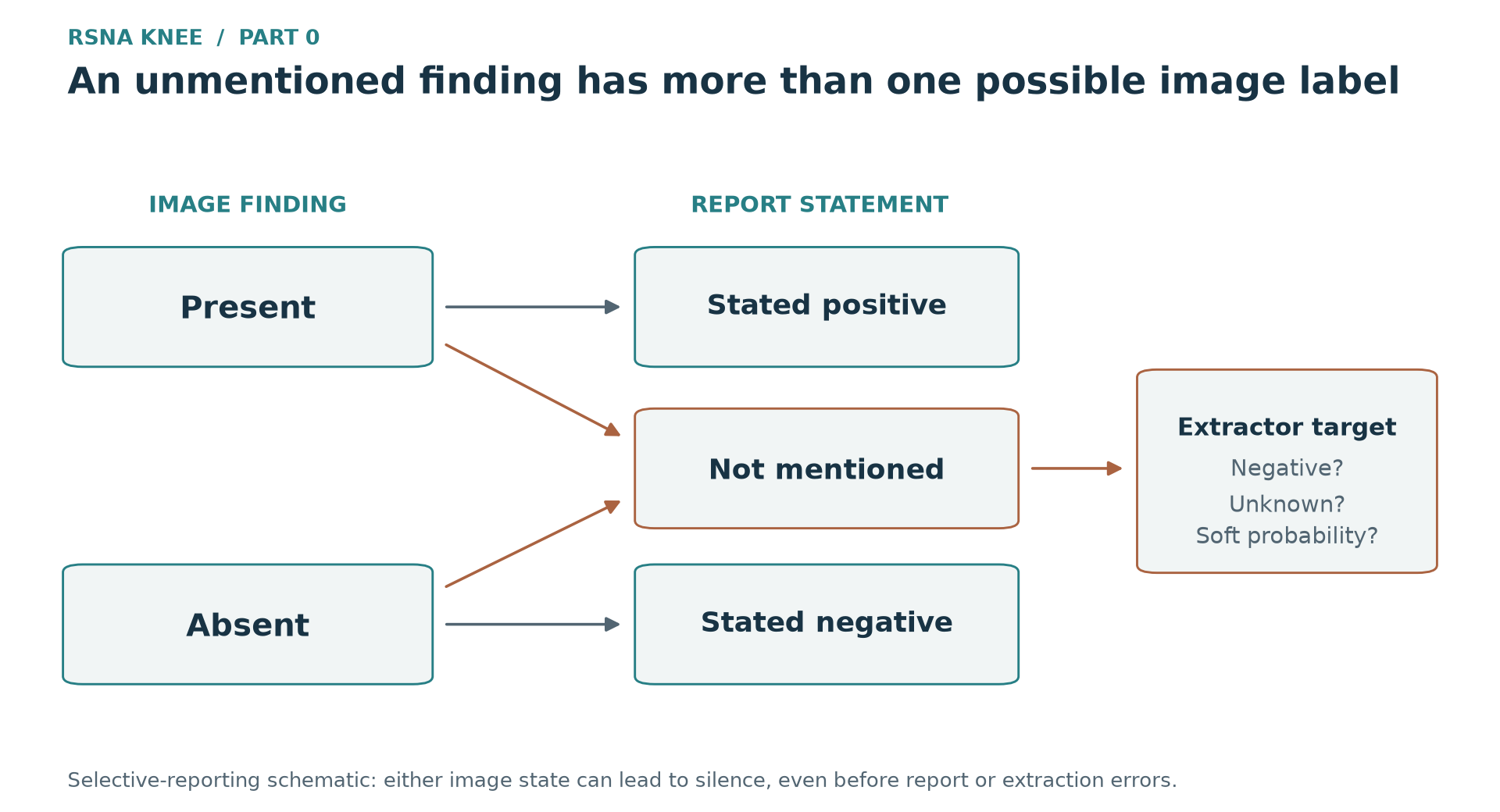
A rule lexicon matches morphology, so its failure mode is silence rather than error: on a phrasing it does not carry it emits no opinion instead of a wrong one. That is also the failure that can be measured without ground truth. For each (report, finding) pair, ask only whether anything matched at all. That rate needs no annotations, so it is available on every study rather than on the few dozen that carry them, and tagged by language it says where the vocabulary is thin.

The two gauges answer different questions and neither substitutes for the other:

	measures	sample	can decide
agreement with annotations	is a fired rule right	58 studies	whether a target’s labels are usable at all
silence rate	does a rule fire	4,407 studies	which language and finding to work on next

Why agreement cannot carry the weight: the Hanley–McNeil standard error of an AUC $A$ with $n_p$ positives and $n_n$ negatives is

\[\mathrm{SE}(A)=\sqrt{\frac{A(1-A)+(n_p-1)(Q_1-A^{2})+(n_n-1)(Q_2-A^{2})}{n_p\,n_n}}, \qquad Q_1=\frac{A}{2-A},\quad Q_2=\frac{2A^{2}}{1+A}.\]

Put $A \approx 0.8$ and a rare finding — a handful of positives among a few dozen studies — into that expression and the standard error lands near $0.09$, a 95% interval of roughly $\pm 0.17$. Competitions are decided by differences an order of magnitude smaller. Choosing between two lexicons on that number is choosing by coin flip, and it will feel like signal every time.

2.2 Reports are graded; annotations are thresholded

The reporting radiologist and the annotator do not share a threshold. A report that says small joint effusion may sit against a negative annotation, because the annotator marked only effusions they judged significant. A rule of the form term present $\Rightarrow$ positive is therefore wrong by construction. Grading the mention — trace, unqualified, marked — is right, and costs nothing, because only the order of the scores is read.

2.3 Nine languages, one lexicon

The extractor identifies no language. Every cue set carries all nine at once and each clause is tested against the union. Routing first means committing to a guess before any evidence is read, and the cheap guess — substring tests, 'the ' for English, 'la ' for French — fails badly, because la is as common in Spanish as in French and whichever test runs first swallows both.

Normalisation comes before segmentation, and it repairs a codepoint problem along the way:

def norm(text):
    """Fold case, diacritics and separators before anything is matched.

    Many Greek reports spell mu with MICRO SIGN U+00B5 rather than U+03BC; NFKD maps one
    onto the other. Turkish dotted and dotless i must be folded before casefolding, or
    'İLİAK' and 'iliak' stop matching.
    """
    t = text.replace("İ", "i").replace("I", "ı").replace("ı", "i")
    t = unicodedata.normalize("NFKD", t)
    t = "".join(c for c in t if not unicodedata.combining(c))
    return re.sub(r"[_\-/]+", " ", t.casefold())

Segmentation attaches a heading line to the value beneath it, because a report that reads Fractures : and then Aucune. states one thing across two lines, and any method that splits them reads a negation as a positive.

Negation is not an edge case. For several findings most mentions are negative, since a report lists what was checked and found intact. Explicit normality counts as negation — ligamentos cruzados y colaterales dentro de límites normales is evidence of absence, not absence of evidence — except where a tear or a high grade is named in the same breath.

Four targets need an anatomy word and a pathology word together. A lexicon of complete phrases carries most matches but cannot survive morphology: Turkish suffixes possessives onto the noun, Croatian and Greek decline it. Where the phrase fails, a second pass matches a stem and requires a side qualifier within a character window:

# A character window rather than a token window, because word order differs: English puts
# the side adjective before the noun and Greek after it.
if re.search(rf"{STEM[t]}.{{0,{W}}}{SIDE[s]}|{SIDE[s]}.{{0,{W}}}{STEM[t]}", clause):
    ...

2.4 The extractor on one report

Below is a report written for this article in the register of the corpus — not taken from it — and what the rule extractor returns for it. The confidence column is the interesting one: 0.05 means no rule fired at all.

IRM DU GENOU DROIT

Ligaments : Le ligament croise anterieur presente une rupture complete avec oedeme
associe. Le ligament collateral medial est intact. Le ligament croise posterieur est
normal.
Menisques : Fissure horizontale de la corne posterieure du menisque interne.
Le menisque externe est sans particularite.
Cartilage : Chondropathie femoro-patellaire de grade II.
Autres : Epanchement articulaire de faible abondance. Pas de fracture.
Petit kyste de Baker.

target	score	conf	what happened
ACL	0.84	0.70	rupture complete with oedema — asserted, high grade
MCL	0.16	0.57	est intact — explicit normality, read as negation
Medial Meniscus	0.84	0.70	fissure + menisque interne matched by stem and side window
Lateral Meniscus	0.28	0.05	missed — sans particularite is a normality phrase the lexicon does not carry
Medial OA	0.28	0.05	not mentioned, correctly silent
Lateral OA	0.28	0.05	not mentioned, correctly silent
PF OA	0.28	0.05	missed — chondropathie femoro-patellaire de grade II did not match
Effusion	0.84	0.70	asserted; faible abondance did not lower the grade
Synovitis	0.53	0.05	not mentioned, silent
Baker’s	0.84	0.70	petit kyste de Baker — asserted
Contusion	0.28	0.05	not mentioned, correctly silent
Fracture	0.16	0.57	Pas de fracture — negated

Two of the twelve are wrong, and both fail the same way: the rule did not fire, and the output is indistinguishable from a finding the report never raised. In a binary extractor that silence would be emitted as a confident negative. Here it is emitted at confidence 0.05, which is what makes it visible — and what makes the corpus-wide silence rate a usable gauge rather than an aesthetic preference.

Note also what did not go wrong: nothing was asserted falsely. That asymmetry is the whole argument for the confidence weight. A silent finding pulls on its output at a quarter of the strength of a spoken one, so the loss is told how much of a claim each target is.

---

3. Reading the acquisition from the header

train_series.csv describes each series with an anatomical plane and two binary flags, Fluid_Sensitive and Fat_Suppression. The names denote two physically independent properties — and that independence is precisely what the delivered columns do not have: across the training series the two agree on every row, so as given they carry one axis between them rather than two.

Both are recoverable from the DICOM header. Fluid sensitivity is a property of the contrast weighting, set by repetition time $T_R$ and echo time $T_E$:

\[\text{weighting} \;=\; \begin{cases} T_1 & T_R \lesssim 800\ \text{ms}\\ T_2 & T_R \gtrsim 800\ \text{ms},\ T_E \gtrsim 60\ \text{ms}\\ \text{PD} & T_R \gtrsim 800\ \text{ms},\ T_E \lesssim 60\ \text{ms} \end{cases}\]

Fluid is bright on $T_2$, intermediate on proton density, dark on $T_1$. Gradient echo breaks the rule — its $T_R$ is short by design — so it is settled by ScanningSequence before the rule is consulted. Fat suppression is a preparation applied on top of any weighting, and is what makes marrow oedema conspicuous: without it the bright fat signal hides it.

Two cautions when reading the description strings, both of which silently invert the answer:

# Underscore is a word character, so a token test for `we` (water excitation) never fires
# inside `t2_de3d_we_tra`. Separators must be normalised to spaces first.
desc = re.sub(r"[_\-.]+", " ", raw.lower())

# ScanOptions must be matched as exact tokens. One vendor writes SAT_GEMS for *spatial*
# saturation, so a substring test for SAT marks non-suppressed series as suppressed.
fatsat = bool(FATSAT_RX.search(desc)) or bool(set(opts.split("\\")) & FATSAT_OPTS)

3.1 Which sequences to show the model

A knee is read in three planes because the structures run in different directions: cruciate ligaments obliquely, best seen sagittally; collateral ligaments and the meniscal body coronally; patellar cartilage and the retinacula axially. Crossing plane with the two acquisition axes gives six slots, chosen so each of the twelve findings has at least one sequence that shows it well.

slot	plane	weighting	fat sat	what it carries
SAG_FLUID_FS	sagittal	PD / T2	yes	meniscal tears, marrow oedema, effusion
COR_FLUID_FS	coronal	PD / T2	yes	collateral ligaments, meniscal body, oedema
AX_FLUID_FS	axial	PD / T2	yes	patellofemoral joint, synovium, effusion
SAG_FLUID_NOFS	sagittal	PD / T2	no	meniscal morphology at high contrast-to-noise
COR_T1	coronal	T1	no	marrow architecture, cartilage and bone outline
SAG_T1	sagittal	T1	no	anatomy, chronic change

A study rarely has all six. A per-slot presence mask carries the absences into the head.

Each panel is the mean of the middle cached slice over 700 studies, so no individual scan is recoverable from it. The femoral condyles and the tibial plateau resolve in the coronal means, the patella in the axial one, the intercondylar notch in the sagittal — which is only possible because the studies underneath were brought to a common scale and orientation first. An aggregate is sharp exactly when the alignment worked.

---

4. Slice order is not file order

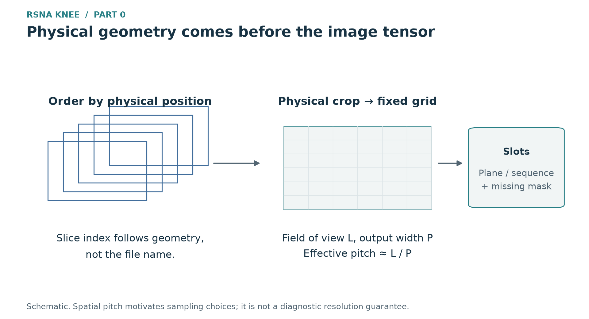
A series is a directory of files, and the obvious way to walk it is to sort the file names. That is wrong, and wrong in a way that produces no error. The file name is the SOP Instance UID — assigned to be unique, not to be ordered.

Left: one sagittal series, plotted as it comes out of a sorted listing. Right: the same slices ordered by their physical coordinate. Over 60 sagittal series the median $|\rho|$ between listing position and physical position is 0.13, with an interdecile range of 0.04–0.28 — indistinguishable from a shuffle.

Three things downstream depend on that order, and all three break silently:

• “Three adjacent slices as three channels.” With an arbitrary order the three channels are three unrelated cross-sections of the knee composited into one image. The encoder is shown a chimera rather than local context.
• “Sample the middle of the stack.” The middle of an arbitrary order is a random subset, not the middle of the joint.
• Reversing slice order to normalise laterality. Reversing a shuffled list produces another shuffled list. The operation does nothing.

The true order is recoverable exactly, and cheaply, from geometry that every slice carries. ImageOrientationPatient gives the in-plane axes $\hat{r}_x, \hat{r}_y$ and ImagePositionPatient the position $\mathbf{p}$ of the first voxel, so

\[\hat{n} \;=\; \hat{r}_x \times \hat{r}_y, \qquad k \;=\; \mathbf{p}\cdot\hat{n},\]

and $k$ increases monotonically along the stack:

ds = pydicom.dcmread(path, stop_before_pixels=True, specific_tags=ORDER_TAGS)
iop = np.asarray(ds.ImageOrientationPatient, float)
ipp = np.asarray(ds.ImagePositionPatient, float)
k = float(np.dot(ipp, np.cross(iop[:3], iop[3:])))

Because $k$ is signed and expressed in patient coordinates, the stack acquires a fixed direction along the body’s left–right axis — which is what the laterality normalisation of §6 reverses, and could not previously have had. InstanceNumber is the fallback where the geometry tags are missing; it usually tracks $k$ up to sign, but interleaved and multi-echo acquisitions number slices in an order that is not the order they occupy in space.

This costs one header read per slice of every chosen series — many more file opens than the pixel decode that follows. On a network mount that cost is latency rather than work, so the ordering pass runs with a wider thread pool than anything else in the pipeline.

---

5. Sampling: how many millimetres one pixel is allowed to be

A DICOM slice of $N \times N$ pixels with spacing $s$ mm/pixel covers $Ns$ millimetres of anatomy. The raw spacing spans 0.167 to 0.562 mm across this corpus, a factor of 3.4 — but that number on its own says nothing, because a higher-resolution acquisition carries proportionally more columns. What survives is the acquired field of view, $Ns$, and it spans 140 to 190 mm between the 5th and 95th percentiles.

That is what a fixed-pixel resize leaves behind. Resizing whole images to 336 px gives an effective pitch of 0.417 to 0.566 mm/pixel — a residual factor of 1.36 — so a meniscus occupies a third more pixels in one study than another for no anatomical reason.

But scale normalisation is only half of it. The other half is a hard limit.

A feature narrower than two pixels does not survive the resize. To represent a structure of width $d$ millimetres the pixel pitch must satisfy

\[s_{\text{eff}} \;\le\; \frac{d}{2},\]

which is the Nyquist condition applied to the resampling grid. A meniscal tear is one to three millimetres, so at $d = 1$ mm the pitch must be at most $0.5$ mm — and if it is not, no capacity downstream recovers the signal, because it was destroyed before the first convolution. This is a property of the resize, not of the network.

Cropping to a constant physical extent $L$ and resampling to $P$ pixels fixes the pitch:

\[n \;=\; \Big\lfloor \frac{L}{s} \Big\rceil \ \text{pixels}, \qquad s_{\text{eff}} \;=\; \frac{L}{P}\ \ \text{mm/pixel}, \qquad \text{token} \;=\; 14\,s_{\text{eff}}\ \ \text{mm}.\]

The pitch is a ratio, so the crop and the resolution trade against each other exactly. At 336 px, a 130 mm crop gives 0.387 mm/pixel and a 100 mm crop gives 0.298 — both under the 1 mm bound, where a 224 px input at 130 mm (0.580) is not.

The crop therefore does two things at once, and the second is easy to miss: it removes the residual 1.36 spread, and it lands the whole corpus at a pitch finer than any of the un-cropped series had — 0.387 against a best case of 0.417.

Two consequences set the numbers:

The crop must be smaller than the smallest field of view, or it silently does nothing. If $L/s$ exceeds the image width the crop cannot be taken and that series passes through unnormalised — quietly, with no error, for as long as nobody checks.

if px and np.isfinite(px) and px > 0:
    want = int(round(CROP_MM / px))
    h, w = shp
    if 16 < want < min(h, w):          # the guard that must be counted, not assumed
        cy, cx = h // 2, w // 2
        half = want // 2
        vol = vol[:, max(0, cy - half):cy + half, max(0, cx - half):cx + half]

Intensity needs the same treatment for the same reason. MR has no absolute scale, so there is no Hounsfield-unit equivalent to anchor to. Each series is normalised to its own 1st and 99th percentile — over the sampled stack rather than per slice, so slices keep their relative contrast, and percentiles rather than extremes, so one bright vessel does not compress everything else.

---

6. Normalising left and right

Four of the twelve targets — the two menisci and the medial and lateral tibiofemoral compartments — are medial/lateral pairs, and a fifth, the medial collateral ligament, is named for the side it lies on. Medial and lateral are defined relative to the body’s midline, so which side of the image they fall on depends on which knee was scanned. Unless that is normalised, those five labels are asked to learn from an axis the model cannot observe.

The correction differs by plane. Coronally and axially the medial–lateral direction lies in the image plane, so flipping the last axis maps one knee onto the other. Sagittally it is the slice axis: each slice is unchanged by mirroring, and what differs is the order in which the stack traverses the joint.

def normalise_laterality(img, plane, lat):
    if lat != "R":
        return img
    if plane in ("Coronal", "Axial"):
        return torch.flip(img, dims=[-1])     # mirror in plane
    return torch.flip(img, dims=[0])          # sagittal: reverse the traversal

Laterality is a Type 2C attribute: it may legitimately be absent, and in this corpus it is absent on half the studies — by whole vendors rather than by scattered series. Leaving those alone is not neutral; it silently declares them left-sided.

The patient coordinate system supplies the missing tag. DICOM patient coordinates are LPS, so $+x$ points to the patient’s left, and the sign of the image centre’s $x$ says which knee this is:

\[c \;=\; \mathbf{p} \;+\; \mathbf{r}\,\Delta_c \frac{N_c}{2} \;+\; \mathbf{d}\,\Delta_r \frac{N_r}{2}, \qquad \text{side} = \begin{cases} \text{right} & c_x < 0\\ \text{left} & c_x > 0\end{cases}\]

with $\mathbf{p}$ the image position, $\mathbf{r}$ and $\mathbf{d}$ the row and column direction cosines, and $\Delta$ the pixel spacing. The centre is used rather than $\mathbf{p}$ itself, which is a corner and sits half a field of view away — enough to change the sign on a knee scanned near the midline.

Two details keep this honest. The median over a study’s series is thresholded rather than any single series, because the header is read from one arbitrary slice per series and a sagittal stack spans the joint. And a study whose centre falls within a short distance of the midline is left unresolved rather than guessed: measured against the studies that do carry the tag, the sign agrees with it on almost all of them and is no better than chance inside that band.

The coronal slot is where the laterality correction is an in-plane mirror, so it is where the effect is visible. Averaged without it, left knees cancel right ones and the medial–lateral asymmetry disappears; the mean gradient rises from 0.870 to 0.902 when they are aligned. On the right, what the physical crop actually removes — not the raw spacing spread, which the matrix size already compensates, but the residual 1.36 in effective pitch that survives a fixed-pixel resize.

---

7. Aggregating six slots into twelve decisions

A study arrives as up to six slot embeddings $x_s \in \mathbb{R}^{d}$ with a presence mask $m_s \in {0,1}$. Pooling them identically would discard the reason the protocol has three planes: each finding is read on particular sequences, and a mean over slots dilutes the one carrying the evidence with five that do not.

Project each slot, add a learned slot identity, give every diagnosis $o$ its own query $q_o \in \mathbb{R}^{H}$, and let it attend over the slots with absent ones masked out of the softmax:

\[h_s \;=\; \phi(x_s) + e_s, \qquad \alpha_{o,s} \;=\; \frac{\exp\!\big(\langle h_s, q_o\rangle / \sqrt{H}\big)\, m_s} {\sum_{s'} \exp\!\big(\langle h_{s'}, q_o\rangle / \sqrt{H}\big)\, m_{s'}},\] \[c_o \;=\; \sum_s \alpha_{o,s}\, h_s, \qquad \ell_o \;=\; \langle c_o, w_o \rangle + b_o .\]

class SlotHead(nn.Module):
    def forward(self, x, mask):
        h = self.proj(x) + self.slot_emb
        att = torch.einsum("bsh,oh->bos", h, self.query) / self.hidden ** 0.5
        att = att.masked_fill(mask.unsqueeze(1) < 0.5, -1e4).softmax(-1)
        ctx = self.drop(torch.einsum("bos,bsh->boh", att, h))
        return (ctx * self.out.weight.unsqueeze(0)).sum(-1) + self.out.bias

The masked softmax renormalises over whatever the study actually contains, so a missing axial series shifts a diagnosis’s attention onto the sequences that are present instead of feeding it a zero vector.

The head is deliberately this small. Richer aggregations are conceivable — attention over every slice group, or a maximum instead of a mean — and there is a structural reason to expect them not to pay: the label is attached to the study, so nothing in the supervision says which part of a study carries the finding. Where the supervision is coarse, so should the aggregation be.

7.1 Why the encoder is trained rather than frozen

A frozen self-supervised encoder is bounded by something no work downstream can reach. Resolution, encoder size, slice coverage and slot aggregation all change how much the model looks and how closely, but none changes the vocabulary it looks with, so every one of those axes runs into the same ceiling. And there is a concrete reason to expect that ceiling to bind here: the encoder learned its features from natural images, where nothing resembles the signal a torn meniscus makes on a proton-density sequence.

So the encoder is adapted, with two restraints. Only the last blocks move — early blocks of a vision transformer are generic edge and texture filters, late blocks are where semantics live, and there may not be enough supervision here to improve the early ones while there is certainly enough to damage them. The encoder learns far more slowly than the head — the head is random at initialisation and has everything to learn, the encoder starts from a good solution and needs only to be moved off it, so the two parameter groups get rates two orders of magnitude apart.

---

8. Reading once, training many times

The cost of this pipeline is dominated by reading, not arithmetic. A study holds several series and each series tens of slices, so a study is on the order of a hundred and fifty files. That is affordable once; it is not affordable once per epoch, and fine-tuning needs the same pixels every epoch. So the slot images are decoded a single time into memory and held as uint8:

\[\text{bytes} \;=\; N_{\text{study}} \times N_{\text{slot}} \times S \times P^{2}\]

with $S$ slices kept per slot at $P$ pixels. The exponent on $P$ is what makes this a real constraint rather than a detail: the cache grows with the square of resolution and only linearly with slices, so coverage is the cheap axis and resolution the expensive one. At 4,407 studies, six slots, twelve slices and 336 pixels that is 33 GB; at 448 pixels it is 59.

What fixes the working configuration is a budget rather than a capacity. The cache is allowed a fraction of the memory reported free, deliberately below the whole of it, because it is the one allocation large enough that overshooting ends the run rather than slowing it — and the encoder, its activations and the buffers in flight are drawn from the same pool.

---

9. Weights are a dataset; the scored run only predicts

Nothing requires the scored run to be the run that learned the weights. A notebook may attach a dataset, weights are a dataset, and the part that genuinely cannot be done in advance is the part depending on studies nobody has seen — reading them, and predicting.

Training inside the scored notebook costs twice: it caps the model at what one accelerator fits inside the time limit, and it spends that time again on every submission for a result that does not change between them.

A package is a list of members, not a model. Each member carries its own weights, its own preprocessing configuration and its own fingerprint. Members are grouped by the pixels they need, each group is decoded once, and a member added later joins the list without changing anything.

A member must prove it is the model it was. Loading a state dictionary succeeds whenever the shapes line up, and shapes line up across every difference that matters — a changed normalisation, a changed resize, a changed slice band. None of those raise. So each member carries the answer it gave to a question generated from a seed, and that answer is recomputed before the member is used:

def fingerprint(model, dev, img_size, n_slot=None, group=None, seed=None):
    """The model's output on a fixed synthetic bag, as a portable identity.

    The input is generated from a seed rather than read, so it is the same on any machine,
    and it is pushed through the whole forward path — the byte scaling, the ImageNet
    normalisation, the resize, the encoder, the slot attention. Any of those differing moves
    the output by order one; numerics differing between two GPUs moves it by about 1e-5,
    which is why the tolerance sits between them rather than at zero.
    """
    g = torch.Generator().manual_seed(seed)
    imgs = torch.randint(0, 256, (2, n_slot, group, img_size, img_size),
                         generator=g, dtype=torch.uint8).to(dev)
    mask = torch.ones(2, n_slot, device=dev)
    mask[1, -1] = 0.0                       # exercise the masked branch of the softmax
    with torch.no_grad():
        return model(imgs, mask, img_size).float().cpu().numpy()

How a member is read. Training draws one group of consecutive slices per step, which doubles as augmentation along the stack. At inference there is no reason to look once, and looking more costs no extra decoding — the cache already holds $S$ slices, so one group from the middle is $1$ forward pass, the disjoint groups are $S/G$, and every consecutive run of $G$ slices is $S-G+1$. Where the average is taken is free but not neutral: averaging logits then squashing is a geometric mean of odds, averaging probabilities an arithmetic mean of risk, and they order studies differently.

---

10. Validating without fooling yourself

Two leaks are specific to this setup, and both inflate a validation number without improving anything.

Shared reports. Some reports are byte-identical across studies — a template read for an unremarkable knee — so every study in such a group receives the same derived target vector. Split the group across the divide and the model is scored on a target whose source it was trained on. Studies are therefore assigned by a hash of the report text, which keeps every duplicate group whole:

grp = np.array([int(hashlib.md5(rep.get(s, s).encode()).hexdigest()[:8], 16) % N_FOLDS
                for s in studies])

Deterministic, no seed, and grouping by report text is implicit and exact: identical report bytes give an identical digest and therefore the same fold.

Two references, two meanings. The holdout covers a fifth of the corpus, measures agreement with the derived targets, and has enough studies per label to separate a real difference from noise — it selects both the epoch within a run and the recipe between runs. The annotation check measures agreement with a radiologist’s reading of the images, which is what the competition scores, but only the annotated studies falling in the holdout can be used and there are very few. It is reported and never allowed to arbitrate: by the standard-error argument of §2.1, a handful of studies gives an interval far wider than the gaps between epochs.

The annotated studies stay in training, at elevated weight, because they are the only labels in the corpus read from the images rather than from text. That choice is exactly why the annotation check must be restricted to the holdout: scoring a model on training examples whose true answers it saw, weighted more heavily than anything else, measures memorisation and reports it as skill.

---

11. What the structure implies

The pipeline is a sequence of decisions that the data forces rather than that taste selects:

decision	forced by
rank averaging, no calibration	AUC is invariant under increasing maps
no text branch	Report exists in train and not in test
grade mentions, never binarise them	the annotator’s threshold is stricter than the radiologist’s
recover both acquisition axes from the header	the delivered flags agree on every row
order slices by $\mathbf{p}\cdot\hat{n}$	file names are identifiers, $	\rho	\approx 0.13$
crop to a constant physical extent	pixel spacing spans a factor of 3.4
$\ge 336$ px at a 130 mm crop	Nyquist for a 1 mm tear
recover laterality from LPS geometry	the tag is absent on half the corpus
per-diagnosis attention over slots	each finding is read on particular sequences
split on a hash of the report text	identical reports give identical targets

The open question is not any one of these. It is that 58 annotated studies cannot arbitrate between two label tables — the interval on the difference is wider than the difference — and the derived labels are what the imaging model is fitted to. That is where the ceiling of this problem sits, and it is a property of the supervision rather than of the network.

---

The notebook is public: RSNA Knee baseline v1. Every figure here is computed from the competition corpus.