Introducing Google Quantum Circuit Compilation
Quantum states, reversible computation, and the invsqrt, DQI, and molecular Hamiltonian tasks: circuit design, resource costs, official verification, and baseline reproduction.
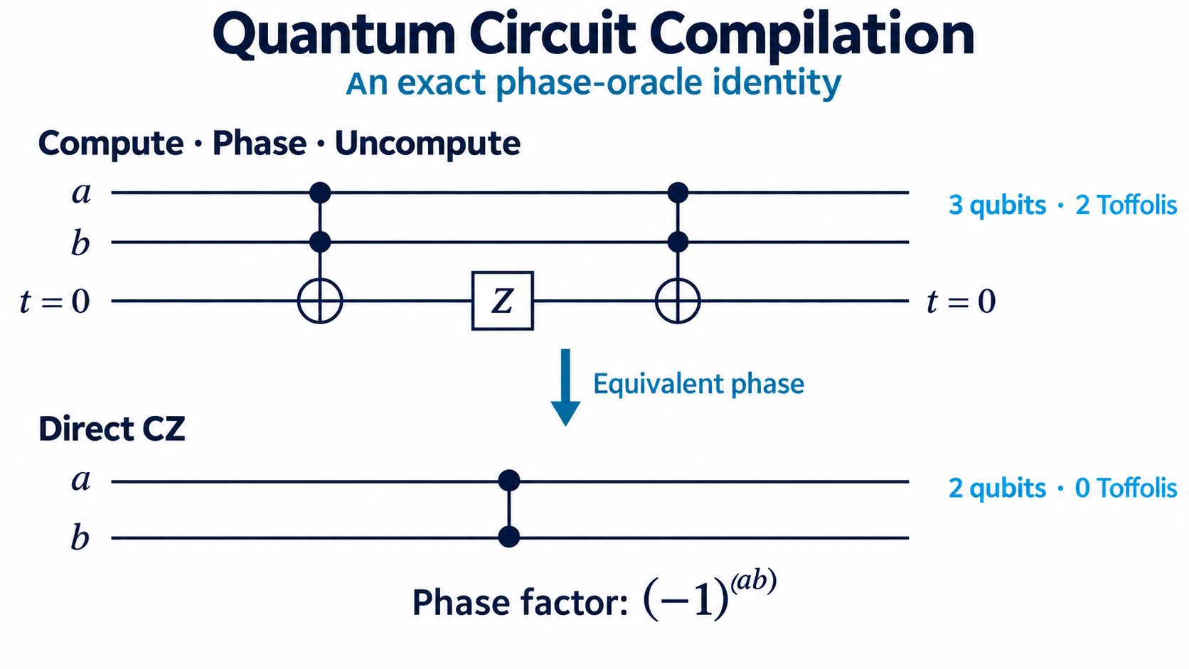
Introduction
Descriptions of quantum algorithms often begin with Fourier transforms, phase estimation, or molecular simulation. Building the actual circuit brings smaller questions into focus. How many qubits does an addition or multiplication need? How many gates does it take to load a number from a table? How can temporary storage be cleared afterward? When these operations repeat many times, they can determine the resources required by the whole algorithm.
Google Quantum AI — Verifiable Quantum Circuit Compilation selects three expensive bottleneck subroutines from quantum algorithms. A bottleneck plays a role similar to a slow function in a classical program, but the resources to reduce include both the operation count and the logical qubits that must remain available during the calculation.
Suppose a subroutine is called 1,000 times and uses 8,000 expensive gates per call. That part alone requires eight million gates. Implementing the same operation with 6,000 gates reduces the total to six million. Qubits can be reused across calls, so their count does not accumulate in the same way as the gate count.
| Full application | Bottleneck isolated by this competition | Why it recurs |
|---|---|---|
| Simulation of Coulomb interactions | invsqrt: a phase proportional to an inverse square root | Interactions must be applied between pairs of particles. |
| Decoded Quantum Interferometry | dqi: Reed–Solomon decoding and phase recovery | Error patterns must be cleaned up inside the optimization algorithm. |
| Molecular electronic-structure simulation | dfthcsos: coefficient factorization, angle lookup, and rotation construction | Operations encoding the Hamiltonian are called repeatedly. |
Each task specifies one subroutine’s inputs, outputs, workspace, and tolerance. The surrounding physics or optimization algorithm remains fixed. Official domain context
1. Separate a qubit’s value, amplitude, and phase
1.1 A bit string now has an amplitude in front of it
A classical bit is either 0 or 1. We write a qubit’s two computational basis states as |0⟩ and |1⟩. The vertical bar and angle bracket denote a quantum state; 0 and 1 name two states that a measurement can distinguish. A single qubit’s pure state can be written as
The complex numbers α and β are probability amplitudes. Measuring in the computational basis returns 0 with probability ∣α∣² and 1 with probability ∣β∣². An amplitude is not itself a probability. Amplitudes can be negative or complex, and they can reinforce or cancel one another. That is what distinguishes the state from a program that merely chooses a random 0 or 1.
A set of n qubits represents n-bit strings. For example, |101⟩ is one basis state of three qubits. A general state includes amplitudes for several strings:
This is superposition. Being able to represent amplitudes for 2ⁿ strings does not mean we can read 2ⁿ answers at once. A measurement returns one of those strings. A quantum algorithm arranges the amplitudes so that useful outcomes become more likely. IBM’s quantum-information lessons develop the notation and operations in more detail.
A group of qubits used to store an integer is called a register. The 22-qubit x register in invsqrt holds an integer. Little-endian means q₀ is the least significant bit: q₀=1, q₁=0, q₂=1 represents 1+0×2+1×4=5. The vertical order of wires in a drawing should not be confused with the place value of the bits.
1.2 Two states with the same measurement probabilities can behave differently
Compare these states:
\[\lvert +\rangle=\frac{\lvert 0\rangle+\lvert 1\rangle}{\sqrt{2}}, \qquad \lvert -\rangle=\frac{\lvert 0\rangle-\lvert 1\rangle}{\sqrt{2}}.\]Measured immediately, both return 0 or 1 with equal probability. Their relative phase differs. The minus sign in |−⟩ multiplies the second amplitude by −1=eⁱπ, a half-turn in phase. A later operation can turn that difference into a measurable difference in probabilities.
The operation we need is the Hadamard gate, H:
\[H\lvert 0\rangle=\lvert +\rangle,\quad H\lvert 1\rangle=\lvert -\rangle, \qquad H\lvert +\rangle=\lvert 0\rangle,\quad H\lvert -\rangle=\lvert 1\rangle.\]Starting at 0 and applying H twice returns to 0. Insert a Z gate between the two H gates to reverse the relative sign, and the final result is 1. Interference has turned a phase difference into an outcome difference.
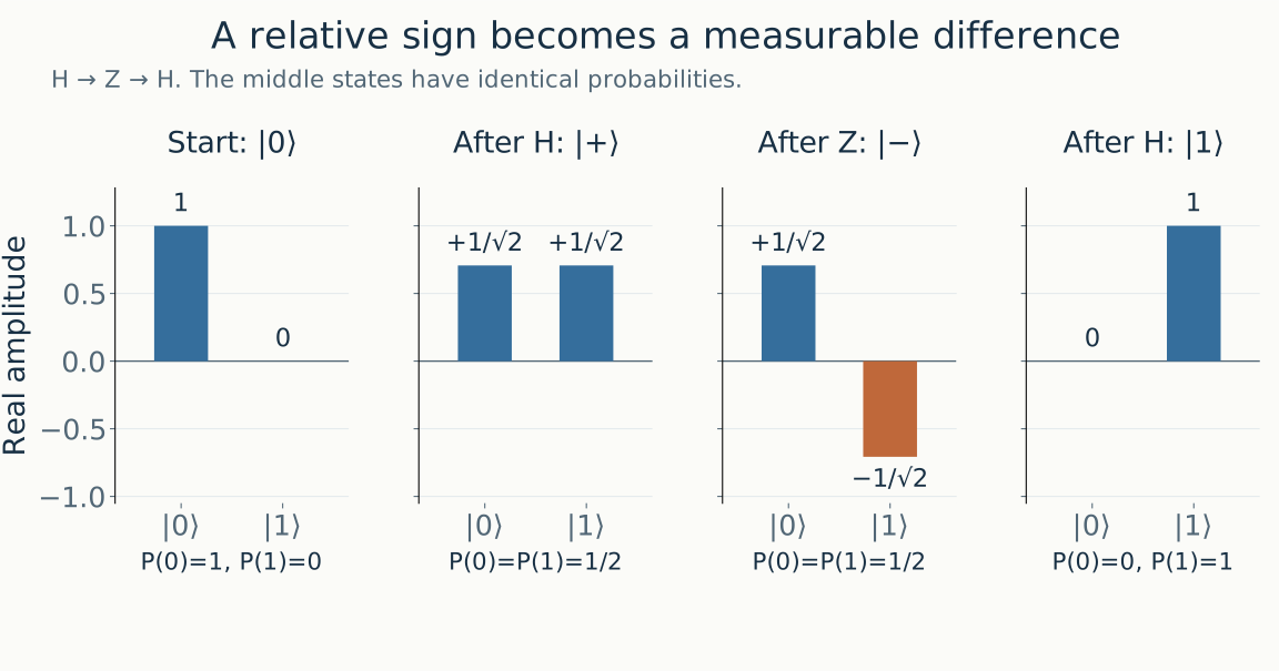
Figure 1. Blue denotes a positive real amplitude and orange a negative real amplitude. Measurement probabilities are unchanged between the state after H and the state after Z, but the final H distinguishes them. Independent H gates are prohibited in submitted kickmix circuits.
At the final H, the amplitude of |0⟩ is (1−1)/2=0, while the amplitude of |1⟩ is (1+1)/2=1: the two contributions cancel in one output and reinforce in the other.
Multiplying the entire state by the same eⁱφ gives a global phase, which does not change measurement probabilities for that state alone. The competition needs phases that depend on the input x. Different terms of a superposition receive different factors, changing their relative phases and therefore the behavior of later operations. Examples of phase and interference
1.3 A quantum circuit is a program that transforms the state in order
In a circuit diagram, each horizontal wire represents a qubit, and gates usually run from left to right. A gate is a small operation acting on one or more wires. In matrix notation, applying a gate means multiplying the state vector by its matrix:
\[X=\begin{pmatrix}0&1\\1&0\end{pmatrix},\quad Z=\begin{pmatrix}1&0\\0&-1\end{pmatrix},\quad H=\frac{1}{\sqrt{2}}\begin{pmatrix}1&1\\1&-1\end{pmatrix}.\]X exchanges 0 and 1. Z multiplies the amplitude of |1⟩ by −1. H mixes the amplitudes of the two basis states. These operations cannot all be understood as bit flips.
| Operation | Action on computational basis states | What matters here |
|---|---|---|
| X | 0 ↔ 1 | Changes a bit value. |
| CX or CNOT | b ← b XOR a | A reversible, controlled bit operation. |
| CCX or Toffoli | c ← c XOR (a AND b) | A building block for reversible AND and arithmetic. |
| Z, CZ, CCZ | Reverse the sign when their conditions hold | The bit values stay the same while the phase changes. |
| Z_POW(q,t) | Multiply the q=1 component by exp(iπt) | Converts a stored number into phase. |
| H | Mix the amplitudes of the two basis states | Useful for explaining the principles; independent H is not a kickmix submission instruction. |
The Z_POW parameter t is measured in half-turns. It differs by a factor of two from turns, where one complete rotation is 1.
2. Why a classical program cannot simply be copied into a quantum circuit
2.1 Use a reversible AND that preserves its inputs
If the result of AND is 0, we cannot tell whether the original input was 00, 01, or 10. Several inputs have merged into one output. Quantum gates without measurement must be reversible, so they cannot discard information this way. Their matrices are unitary and have inverses.
The basic solution is to preserve the input and XOR the result into a separate target bit:
\[U_f:\lvert x\rangle\lvert z\rangle\longmapsto\lvert x\rangle\lvert z\oplus f(x)\rangle.\]When z starts at 0, the target becomes f(x). Apply the same XOR again and it returns to z. CCX(a,b,c) is the case f(a,b)=a AND b.
| a | b | Initial c | c after CCX | c after a second CCX |
|---|---|---|---|---|
| 0 | 0 | 0 | 0 | 0 |
| 0 | 1 | 0 | 0 | 0 |
| 1 | 0 | 0 | 0 | 0 |
| 1 | 1 | 0 | 1 | 0 |
Addition and multiplication are also built from reversible components. Classical code can overwrite the old a in a *= b. A reversible implementation must specify which information remains and what must be restored. Carries, partial products, and comparison results all occupy temporary qubits. Constructing reversible classical computation
2.2 Leftover temporary values obstruct interference
A temporary qubit is called an ancilla or a scratch qubit. It usually has to return to 0 after its job is done. This is about more than tidy memory management.
Suppose the first qubit is |+⟩ and a CX writes its basis value into a second, temporary qubit:
The CX copies computational-basis values. The right side is not two independent |+⟩ states, so this does not clone an arbitrary quantum state. The two qubits are entangled. The temporary qubit now carries information distinguishing the two branches. If we ignore it, the first qubit no longer interferes as the original |+⟩ would. Applying H to the original state would always produce 0; leaving the temporary information in place gives the first qubit equal probabilities for 0 and 1.
A test that checks only whether x has the correct bit value on one basis input can miss this distinction. The verifier therefore checks register restoration, clean workspace, and phase together. A smaller file or gate count is no improvement if it breaks these requirements.
2.3 Compute, apply phase, then uncompute
When the required effect is a phase proportional to f(x), as in invsqrt, we can use this pattern:
Here f(x) is actually an approximation represented with finitely many bits. The final uncomputation restores the bit values while leaving the input-dependent phase in place. Reversing a sequence requires applying each gate’s inverse in reverse order. X, CX, and CCX are their own inverses; a general rotation requires negating the angle.
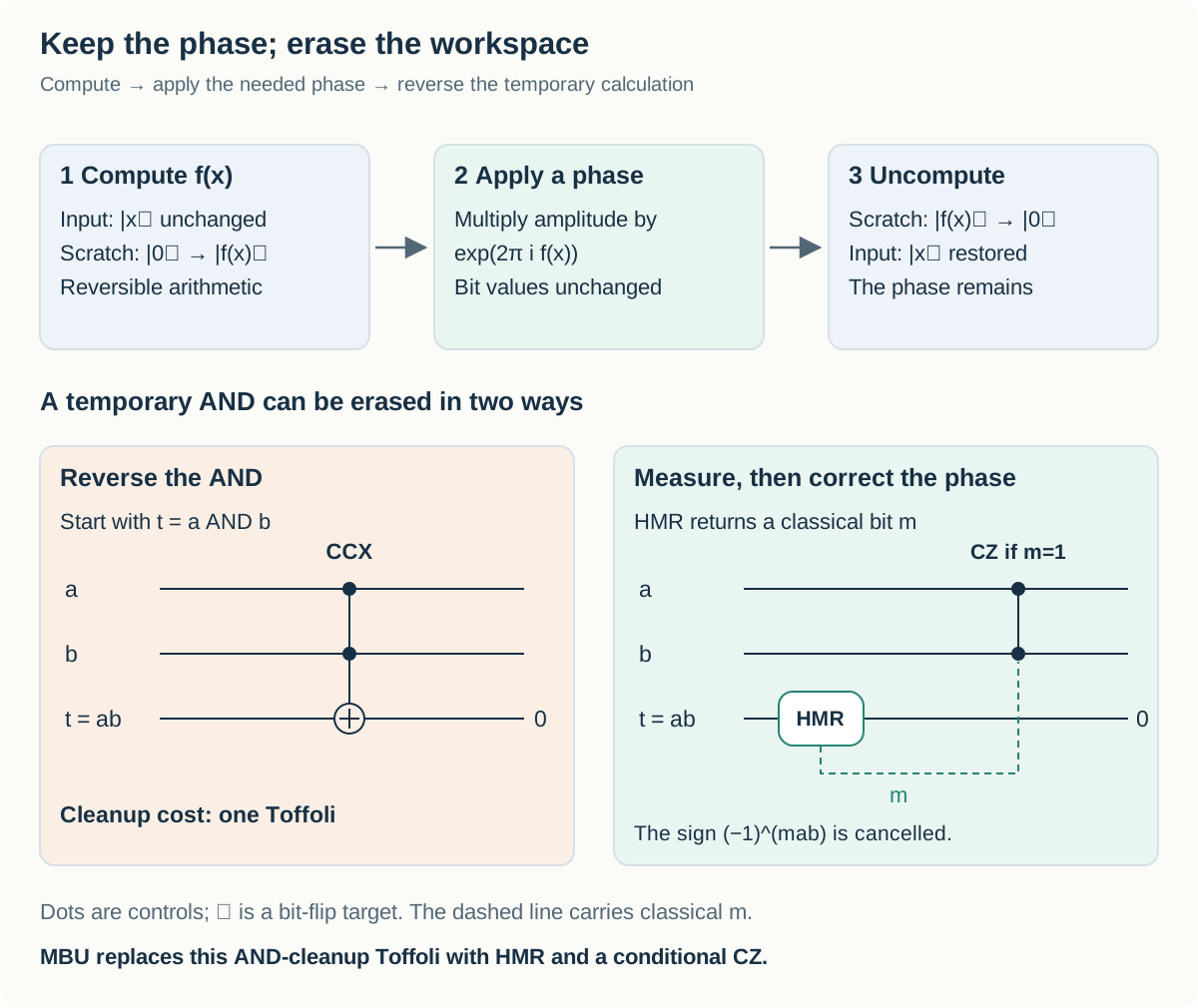
Figure 2. The upper path clears workspace while retaining the phase. The lower paths show two ways to erase a temporary AND. Dots are controls, ⊕ is a bit-flip target, and the dashed wire carries a classical measurement bit. The HMR path includes a phase correction controlled by its measurement result. Arbitrary computed values cannot always be erased for free.
2.4 How measurement-based uncomputation saves a Toffoli
Clearing t=a AND b with another CCX costs one Toffoli. Another method uses HMR: measure t in the X basis and reset it to 0. If the measurement result is m, it introduces this sign:
When m=0, no correction is needed. When m=1, applying CZ(a,b) adds another $(-1)^{ab}$ factor, cancelling the unwanted sign. The conditional CZ costs no Toffoli in this model. The measurement and phase correction together implement measurement-based uncomputation, or MBU.
Omitting the measurement or its correction changes the circuit. Forcing a dirty qubit to 0 with R is not a valid shortcut either. R is intended to release workspace already cleaned to 0; the simulator makes incorrectly discarded information show up as a random phase. The kickmix documentation defines the instruction semantics.
Some temporary values are cheaper to erase through measurement and correction, while others require an expensive correction. Keeping a value for longer can increase Q. Erasing it early and recomputing it later can increase the gate count. Designing a reversible circuit means balancing these choices across the whole calculation.
3. What does compilation need to make cheaper?
3.1 Mathematics, integer algorithms, and gates are different layers
The instruction “calculate 1/√x” does not determine a circuit. We still need to choose the fractional precision, approximation polynomial, multipliers, and cleanup schedule. That is why the same mathematical operation has many circuit implementations.
| Layer | Example for invsqrt | Design choices |
|---|---|---|
| Required behavior | Apply an inverse-square-root phase depending on x | Fixed by the competition contract. |
| Numerical algorithm | Normalization, approximation, Newton correction | Polynomial degree, interval count, correction steps. |
| Integer implementation | Fixed-point multiplication, addition, shifting | Bit precision, truncation, register reuse. |
| Reversible gates | CX, CCX, phase operations, MBU | Adder design, AND cleanup, workspace lifetime. |
| Error-corrected hardware | Implement logical gates with physical operations | Not directly executed or optimized in this competition. |
Compilation here extends beyond translating source-language syntax into machine instructions. It includes choosing a numerical algorithm and reversible implementation within a correctness limit. Faster classical code generation and a lower official cost for the generated quantum circuit are separate outcomes.
3.2 Logical qubits and expensive gates
The competition’s Q counts logical qubit resources under an error-corrected model. Protecting one logical qubit on hardware can require many physical qubits. Q=260 therefore does not mean 260 physical devices. Estimating hardware size also requires a physical error rate and an error-correction scheme.
Gates do not all have the same cost either. Non-Clifford operations such as Toffoli matter in this competition; invsqrt converts four T gates into one Toffoli equivalent. Arbitrary-angle rotations receive a synthesis cost that depends on the required accuracy. The Clifford family includes X, CX, Z, and H; T and Toffoli lie outside it. T multiplies the $\lvert 1\rangle$ component by $e^{i\pi/4}$. A Clifford operation treated as free in the official formula still takes some resources on real hardware.
For the invsqrt resource product,
Reducing qubits by 10% while increasing the equivalent gate cost by 5% changes the product to 0.9×1.05=0.945: a 5.5% reduction. Reducing gates by 10% while adding 20% more qubits gives 0.9×1.2=1.08, making the cost worse. Candidate circuits must also pass correctness verification.
4. Why can a classical CPU verify these circuits?
4.1 Follow basis-input trajectories instead of storing the whole superposition
Representing a general n-qubit state directly can require 2ⁿ amplitudes. kickmix instead restricts the circuit to reversible classical gates, diagonal phases, and measurement-based cleanup. Starting from one computational basis input, the simulator follows one bit string, a phase, and measurement records. CX updates a stored bit through XOR; Z changes the phase sign when its condition holds.
An independent H, used earlier to explain interference, would spread one basis input over several basis states and is not an allowed submission instruction. HMR is a particular measurement-and-cleanup operation with specified semantics and a specified trajectory model. The complete quantum algorithm has not become classically easy; an expensive part of it has been isolated in this restricted form.
For a clean phase circuit without measurements, the correct action on every basis input determines its action on a superposition by linearity:
\[\sum_x\alpha_x\lvert x\rangle\lvert 0\rangle \longmapsto \sum_x\alpha_x e^{2\pi i f(x)}\lvert x\rangle\lvert 0\rangle.\]Actual verification must also account for approximations and measurement branches. The companion paper connects sampled failure rates to quantum-state error under assumptions about input weighting and the structure of each branch. A passing result should not be interpreted as a formal proof applicable to any quantum circuit.
4.2 Three checks within a verification shot
One simulation trial is called a shot. The verifier prepares an input, runs the circuit, and checks the following:
| Check | What could go wrong if it were omitted? |
|---|---|
| Do input and output registers match the contract? | A circuit could apply the right phase while corrupting x or the syndrome. |
| Does scratch return to 0? | Leftover intermediate values could disrupt interference between branches. |
| Is the accumulated phase within tolerance? | The bits could be correct while the effect required by the quantum algorithm is wrong. |
invsqrt tests every x 64 times, but does not enumerate every possible measurement record. DQI tests error patterns drawn from a specified distribution. The chemistry task checks ANGLE outputs and uncomputation by address, then combines those results with the numerical data to calculate the total cost. PASS therefore has a different testing scope in each task.
4.3 Circuit hashes, private salts, and local reproduction
Test randomness is derived from a SHA-256 digest of the submission content and a salt. invsqrt hashes a canonical binary circuit; the chemistry task also incorporates data such as the factorization and tree. Kaggle’s Public and Private evaluations use different private salts. The design makes it harder to memorize a small, fixed set of public random test inputs. The official metric defines the details.
Repeating the same circuit with the same salt repeats the same pseudorandom samples; it does not add independent evidence. Changing the circuit changes its hash, producing a different stream even with the same salt. If conditional gate counts or failure rates depend on measurement outcomes, the measured cost can change too.
Full local verification completes the official task’s full test workload using the recorded files, settings, and local environment. Kaggle parity depends on its binary and salts; sampled measurement branches remain a statistical check.
5. invsqrt: turn an inverse distance into phase
5.1 Why does fusion simulation need an inverse square root?
A fast charged particle loses kinetic energy as it travels through matter and interacts with nearby electrons. The energy lost per unit distance is called stopping power. Predicting where particles deposit energy in fusion fuel requires calculating electronic motion in hot, dense matter. The competition isolates an arithmetic circuit called repeatedly inside that simulation. Rubin and colleagues’ original research provides the scientific background.
For electrons at positions $\mathbf r_i,\mathbf r_j$, the magnitude of the Coulomb interaction is inversely proportional to their separation. Omitting units and physical constants,
\[V_{ij}\propto \frac{1}{\lVert\mathbf r_i-\mathbf r_j\rVert} =\frac{1}{\sqrt{(x_i-x_j)^2+(y_i-y_j)^2+(z_i-z_j)^2}}.\]Calling the squared distance x leaves the function $1/\sqrt{x}$. When time evolution is approximated in small steps, the position-dependent potential energy enters as a position-dependent phase change. The general time-evolution factor is $e^{-iV\Delta t/\hbar}$; the competition defines its own contract with the units, sign, and scale fixed.
There are $\binom{218}{2}=23{,}653$ distinct pairs among 218 electrons. Calling the same operation tens of thousands of times per time step allows a small saving per call to accumulate across the simulation. That is how a seemingly simple function becomes a scientific-computing bottleneck. Official domain context
5.2 The output is a phase, not a number register
A classical program might write return 1 / sqrt(x) and return an approximate number. This circuit has a different final interface. It preserves the input number and multiplies its amplitude by a phase. Every temporary qubit must end at 0:
Here |x⟩ denotes the integer stored in 22 qubits. If the input is a superposition of several integers, each term receives its own phase. For example, 4 receives half a turn and 16 receives a quarter-turn:
The probabilities of measuring 4 and 16 immediately after this operation are still equal. What changed is their relative phase. Later operations can turn that difference into interference. Correct output bits with an incorrect phase therefore do not make a correct circuit. A factor that looks like global phase when inspecting one basis input must be matched consistently across a superposition of inputs.
The reference circuit first computes an approximation in workspace, uses its bits to apply phase, then reverses the arithmetic to clear the workspace. Reading the circuit as compute → phase → uncompute makes its long sequence easier to follow:
\[\lvert x\rangle\lvert 0\rangle \xrightarrow{\text{compute}} \lvert x\rangle\lvert \widetilde f(x)\rangle \xrightarrow{\text{phase}} e^{2\pi i\widetilde f(x)}\lvert x\rangle\lvert \widetilde f(x)\rangle \xrightarrow{\text{uncompute}} e^{2\pi i\widetilde f(x)}\lvert x\rangle\lvert 0\rangle.\]The official input/output contract is:
| Requirement | Official instance |
|---|---|
| Input x | 1…3,133,452 |
| Input register | One little-endian x of 22 distinct qubits; no other named registers |
| Target phase | 1/√x turns at β=1, compared modulo one turn |
| Tolerance | 2⁻²⁴/√x turns |
| Cleanup | Restore x and return every other qubit to zero |
| Workload | 64 shots for every x, 200,540,928 in total; no failures allowed |
5.3 Fixing the binary point turns fractions into bit strings
A reversible circuit cannot simply call Python’s floating-point arithmetic. The reference uses fixed-point arithmetic: integer bit strings whose binary-point position is agreed in advance. With F fractional bits, stored integer Y represents $Y/2^F$. For instance, 0011 with four fractional bits stores integer 3 and represents $3/16=0.1875$.
More bits improve precision, but multiplication then needs more partial products, additions, and workspace. The circuit does not compute every intermediate to the final precision. It uses column-truncated multiplication, omitting low-weight partial-product bits that will be discarded. Truncating each partial product is different from doing an exact multiplication and rounding the complete result once at the end.
The official generator’s Precision configuration sets five widths independently:
| Value in the pipeline | Fractional precision | Purpose |
|---|---|---|
Polynomial input offset delta | 14 bits | Locates the input within a small interval. |
| Coefficients, Horner intermediates, initial value $y_0$ | 17 bits | Produces a relatively cheap initial approximation. |
| $y_0^2$ | 28 bits | Supplies the square for Newton correction. |
| $My_0^2$, $3-My_0^2$ | 28 bits, plus 2 integer bits | Calculates the correction factor. |
| Final product $p$ | 29 bits, plus 1 integer bit | Stores the corrected value. |
| Phase word $Y$ | 40 bits in total | Incorporates normalization and the final factor of $1/2$. |
5.4 First, reduce the large input range to [1, 4)
The input domain is $1\le x\le3{,}133{,}452$. Applying a uniform absolute precision across this whole range would also store the leading fractional zeros of small results, making the multipliers wider. The reference counts leading 00 pairs in the input, calls their number s, and shifts left by two bits per pair. Distinguish the integer held in the register from the normalized real number it represents:
A hand calculation for $x=64$. Its 22-bit representation contains 15 zeros before the seven significant bits. That gives seven leading 00 pairs, so $s=7$. Shifting left by 14 bits produces $x_{\rm norm}=64\times2^{14}=2^{20}$, hence $M=1$. Restoring the scale gives $2^{7-10}/\sqrt1=1/8$. This is the ideal normalization result; the reference then applies fixed-point approximations.
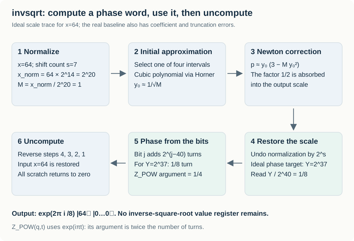
Figure 3. Normalization maps x=64 to M=1 with s=7. In ideal arithmetic, the final 40-bit phase word is $2^{37}$, representing $1/8$ turn. The pipeline then clears its workspace. The reference uses truncated coefficients and products, so its stored word can differ from this ideal value.
Since s depends on the input, the quantum circuit must store it too. The reference uses ten flag qubits. Seven is represented by seven true flags—a unary representation—rather than the usual binary 0111. Each flag later controls one shift.
5.5 Obtain a cheap initial estimate, then correct it once
After normalization, the circuit makes initial approximations on four small intervals: [1, 1.5), [1.5, 2), [2, 3), and [3, 4). Leading bits select an interval and its cubic-polynomial coefficients. The upper two intervals reuse appropriately rescaled coefficients from the lower intervals, using the $1/\sqrt2$ relation.
A polynomial $c_0-c_1\delta+c_2\delta^2-c_3\delta^3$ can be evaluated with the following nesting. This is Horner’s method: three successive multiplications replace separately computing $\delta^2$ and $\delta^3$.
\[y_0=c_0-\delta\bigl(c_1-\delta(c_2-c_3\delta)\bigr) \approx\frac1{\sqrt M}.\]Here $\delta=M-a$, where $a\in{1,1.5,2,3}$ is the selected interval’s left endpoint; the circuit retains 14 fractional bits of this offset.
The initial estimate does not need to supply all the final accuracy on its own. One Newton update can greatly reduce a small approximation error:
\[y_{\rm next}=\frac{y_0}{2}(3-My_0^2).\]Why is one correction useful? In ideal arithmetic without rounding or truncation, substitute $y_0=(1+e_0)/\sqrt M$. The new relative error becomes
\[e_1=-\frac32e_0^2-\frac12e_0^3.\]An initial relative error of $10^{-4}$ becomes approximately $1.5\times10^{-8}$ in magnitude. A small error is roughly squared. This formula excludes fixed-point truncation, however. The actual circuit must be checked with polynomial approximation, coefficient quantization, and every truncated multiplication included.
The official generator does not multiply by $1/2$ explicitly. It computes $p\approx y_0(3-My_0^2)\approx2/\sqrt M$. Its stored integer p has 29 fractional bits, is shifted by s to produce Y, and is finally interpreted as $Y/2^{40}$. The factor of $1/2$ is absorbed into the output binary point. For x=64 and M=1, write the ideal real-valued target as $p_=2$. Its final phase-word target is $Y_=2^{29}p_2^7=2^{37}$, giving $Y_/2^{40}=1/8$. The actual p register has 29 fractional bits and one integer bit, 30 bits in total, so it represents values below 2. The boundary value 2 belongs to the ideal calculation; the stored, truncated value must satisfy the tolerance.
5.6 Apply phase bit by bit, then clear the calculation
If $Y=\sum_{j=0}^{39}b_j2^j$, the required phase is $Y/2^{40}=\sum_jb_j2^{j-40}$ turns. A rotation of $2^{j-40}$ turns conditioned on each set bit $b_j$ adds up to the desired phase. This decomposes a large phase operation into small controlled phases.
The actual Z_POW argument is in half-turns, so the code passes $2^{j-39}$. Z_POW q t multiplies the $\lvert 1\rangle$ component by $e^{i\pi t}$: to apply $2^{j-F}$ turns, use $t=2^{j-F+1}$. Confusing turns with the argument’s unit causes a factor-of-two error.
After applying phase, the circuit reverses the shifts, Newton arithmetic, polynomial evaluation, interval selection, and input normalization. The input x returns to its original integer, and scratch—including Y—returns to 0. The phase remains. Discarding a temporary value and uncomputing it are different operations.
5.7 Where does the reference spend its gates?
Static Toffoli counts by tagged section of the supplied invsqrt.kmb:
| Stage | Compute direction | Uncompute direction | What it does |
|---|---|---|---|
| Normalization | 120 | 110 | Tests leading zeros and controls shifts. |
| Interval selection | 3 | 0 | Uses MBU to clear selector flags. |
| Three Horner multiplications | 1,071 | 1,071 | Builds the initial approximation. |
| $y_0^2$ | 442 | 442 | Exploits the symmetry of a square. |
| $M y_0^2$ | 1,043 | 1,043 | A substantial arithmetic cost. |
| $3-z$ | 28 | 28 | Forms the correction through subtraction. |
| $y_0(3-z)$ | 867 | 867 | Performs the final correction multiplication. |
| Denormalization | 300 | 300 | Restores the scale with controlled shifts. |
| Total | 3,874 | 3,861 | 7,735 combined. |
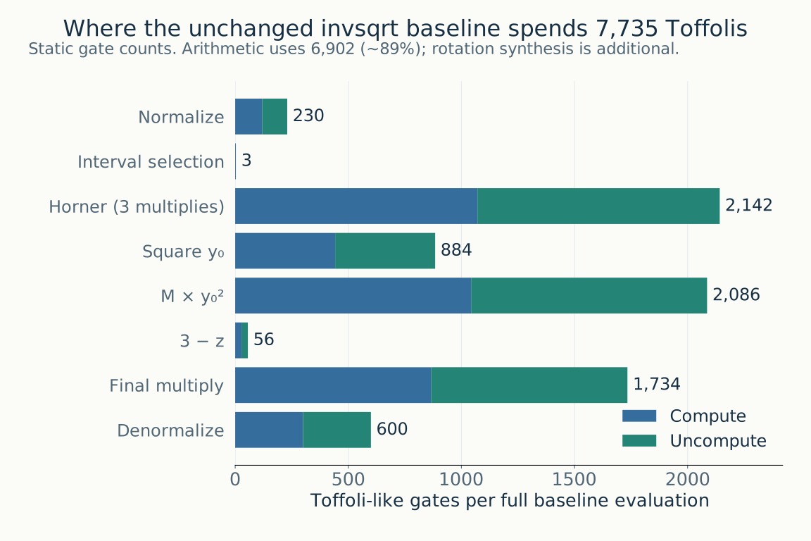
Figure 4. The original reference contains 7,735 Toffoli-like gates, split between compute and uncompute. Rotation-synthesis costs are added separately when calculating the final Toffoli-equivalent cost.
Multiplication, squaring, and subtraction together account for 6,902 gates in both directions, approximately 89% of the total. Changing the arithmetic structure or precision is therefore more likely to change the quantum cost directly than reducing Python function calls. Phase-rotation synthesis adds further cost: about 253 Toffoli equivalents in the existing local result.
del_and already uses measurement-based cleanup for temporary ANDs. In both directions, _add_row builds partial-product ANDs, performs an addition or subtraction, and clears those ANDs through measurement. Restoring carries and an earlier accumulator cannot automatically be made free in the same way as erasing one temporary AND.
5.8 Precision is both an acceptance condition and a cost variable
For every valid x, phase error must be no greater than $2^{-24}/\sqrt{x}$ turns. As x increases and the target phase shrinks, the allowed absolute error shrinks too. Matching a few small inputs is insufficient. The official test runs every input 64 times—200,540,928 shots in total—and checks input restoration, zero scratch, and phase.
Synthesizing small-angle phase gates into an error-corrected gate set introduces error and cost. After checking arithmetic error, the verifier assigns the smallest remaining margin to synthesis error. Removing one precision bit may reduce Toffolis but increase arithmetic error, leaving less margin and making rotation synthesis more expensive. Using up the entire arithmetic tolerance can leave no synthesis margin and cause rejection. The comparison must use the final cost of an accepted circuit, rather than its Toffoli count alone.
5.9 What should a first candidate change?
| Approach | Mechanism | What to check first |
|---|---|---|
| Reuse workspace qubits | Values with nonoverlapping lifetimes share logical wires. | Exactly when the old value is cleaned to 0; input preservation. |
| Adjust intermediate precision | Omit unnecessary low-weight partial products and carries. | Worst-case error near interval boundaries and at large x; synthesis margin. |
| Redesign the initial approximation | Change interval count, polynomial degree, and lookup size together. | Whether a cheaper initial estimate requires wider Newton arithmetic. |
| Change the shift network | Implement unary-controlled shifts with another control structure. | Savings after computing and clearing the control bits are included. |
| Change arithmetic decompositions | Replace reversible multipliers, squarers, or adders. | Carries, overflow, signedness, and truncation semantics. |
Change one mechanism at a time and test against the original circuit under the same contract. Changing precision, polynomials, and wire placement simultaneously would make a success or failure harder to explain.
The concrete contract and implementation are in verifiers/invsqrt/verify_submission_invsqrt.py and nr_reference_circuit.py in the official competition data. The companion paper’s Benchmark I discussion provides the broader setting; the scales and bit widths above follow the supplied code.
Read Precision → _compute_y1 → _phase_by_bits → build_nr_circuit in nr_reference_circuit.py. Within _compute_y1, _normalize, _horner, _square, _multiply_m, _correct, _multiply_y0, and _denormalize match the stages above. The separate fixed_point_model is a numerical model, distinct from generated-circuit verification.
6. DQI: why an optimization algorithm needs an error decoder
dqi seeks good polynomials in a combinatorial optimization problem. The submitted quantum subroutine removes the record of an error pattern while preserving a superposition.
6.1. Start with polynomial fitting over a finite field
In ordinary curve fitting, we look for a real-valued polynomial close to observed points. In Optimal Polynomial Intersection (OPI), each evaluation point over a finite field has a set of allowed values. A coefficient vector $x$ defines a polynomial $p_x$; the objective counts how often its evaluations land in the allowed sets.
\[p_x(z)=\sum_{k=0}^{n-1}x_kz^k, \qquad f(x)=\left|\{j:p_x(\alpha_j)\in F_j\}\right|.\]Here $F_j$ is the set of allowed values at evaluation point $\alpha_j$. Given a candidate, we can check its quality by evaluating $f(x)$. Finding a good candidate and checking a candidate’s score can have very different computational costs. DQI builds a quantum probability distribution in which good candidates are measured more often. The original OPI and DQI paper
Conceptually, the final DQI state has the form
\[\lvert \psi\rangle\propto\sum_x P(f(x))\lvert x\rangle, \qquad \Pr[x]\propto|P(f(x))|^2.\]The polynomial $P$ is chosen to give larger amplitudes to desirable objective values. The challenge is preparing this state. DQI uses a Fourier transform to turn that task into one involving sparse error patterns and their syndromes. A syndrome is a compact algebraic summary of an error vector.
6.2. Error decoding becomes a way to erase a quantum register
Write the linear map that computes a syndrome as $B^T$. A central step has the following structure:
\[\sum_e a_e\lvert e\rangle\lvert B^Te\rangle \ \longrightarrow\ \lvert 0\rangle\sum_e a_e\lvert B^Te\rangle.\]On the left, error pattern $e$ is entangled with its syndrome $B^Te$. To produce the desired interference, the algorithm must erase the error register before applying a Fourier transform to the remaining syndrome register. Measuring the error pattern in the computational basis would reveal which component is present and would not preserve the required superposition. Instead, a reversible decoder reconstructs the error from the syndrome and XORs it into the original register: $\lvert e\oplus e\rangle=\lvert 0\rangle$. This is where error-correcting-code decoding enters the algorithm.
Under a bound on the number of errors, the syndrome determines the error pattern uniquely. The competition’s Reed–Solomon code has length 4,095, dimension 4,025, and minimum distance 71. It can therefore correct up to 35 symbol errors. This is not a limit of 35 flipped bits. Each symbol contains 12 bits; at most 35 symbol positions have a nonzero value.
The DQI construction saves qubits by generating error symbols one at a time and erasing them through X-basis measurements. This measurement-based uncomputation (MBU) saves workspace but leaves a measurement-dependent sign on each component of the superposition. The decoder must reconstruct enough information about the hidden error pattern to cancel those signs. Reversible decoding and the MBU construction
6.3. GF(2¹²) arithmetic is not integer arithmetic modulo 4,096
The official circuit works over the finite field $\mathrm{GF}(2^{12})$, which has 4,096 elements. Although each element is represented by 12 bits, multiplication is not ordinary integer multiplication followed by reduction modulo 4,096.
Read a bit string $(a_0,\ldots,a_{11})$ as the polynomial $a_0+a_1u+\cdots+a_{11}u^{11}$. Addition is coefficient-wise arithmetic modulo 2: XOR. Multiplication means multiplying these polynomials and taking the remainder after division by a fixed irreducible polynomial. The official representation uses a little-endian polynomial basis and the modulus
\[u^{12}+u^6+u^4+u+1.\]| Operation | Meaning at the bit level | Consequence for circuit design |
|---|---|---|
| Addition of two field elements | Bitwise XOR | Can be implemented with CNOTs |
| Multiplication by a fixed field constant | A linear transformation over GF(2) | Can be implemented as a CNOT network |
| Multiplication of two quantum field registers | A bilinear computation depending on both inputs | Requires Toffoli resources |
| Inversion of a nonzero element | Computing $a^{-1}$ | Requires a multiplication chain and workspace |
Even within “multiplication,” the cost depends strongly on whether one operand is known at compile time. This is one reason the fastest decoder on a CPU need not give the cheapest quantum circuit.
6.4. Actual inputs and outputs: the error vector is withheld
Write the error vector as $e=(e_0,\ldots,e_{4094})$ and the field’s primitive element as $\alpha$. Rather than supplying the error vector, the verifier supplies 70 syndromes:
\[S_i=\sum_{j=0}^{4094}e_j\alpha^{(i+1)j}, \qquad i=0,\ldots,69.\]The sum is field addition, which is XOR in the binary representation. Registers $S_0,\ldots,S_{69}$ each contain 12 qubits, for 840 input qubits in total. Each position also has a measurement mask $M_j$ consisting of 12 classical bits. The official registers named E0 through E4094 hold these masks. Despite their names, they do not contain the hidden errors $e_j$.
The required operation is
\[U_M\lvert S(e)\rangle\lvert 0\rangle_W =(-1)^{b(e,M)}\lvert S(e)\rangle\lvert 0\rangle_W, \quad b(e,M)=\left(\sum_j\operatorname{popcount}(e_j\mathbin{\&}M_j)\right)\bmod2.\]Here & means bitwise AND and popcount counts set bits. This expression does not take a field product. It computes the parity of the selected error bits: odd parity contributes −1, even parity +1. The syndrome must be restored to its original value, and every additional qubit must return to zero. The circuit does not have to leave the decoded error vector in an output register. This allows implementations that compute the required phase without retaining every error value.
For a single fixed basis input, this looks like an overall sign. But the sign varies with $e$. Across a superposition, it becomes a relative phase between components and changes the measurement distribution after the next Fourier transform.
The register interface must be exactly S0…S69 as disjoint 12-qubit registers and E0…E4094 as disjoint 12-bit classical registers, with no other named registers. The DQI verifier also prohibits Z_POW instructions. The official data contain verifiers/dqi/verify_submission_dqi.py, which defines this contract.
6.5. A GF(4) example that fits on paper
For an RS(3,1) code with one symbol error, use the elements ${0,1,\alpha,\alpha+1}$ with $\alpha^2=\alpha+1$.
| Element | Polynomial | Bits, most significant first |
|---|---|---|
| 0 | 0 | 00 |
| 1 | 1 | 01 |
| $\alpha$ | $u$ | 10 |
| $\alpha^2$ | $u+1$ | 11 |
In this field, $\alpha^3=1$ and $\alpha+\alpha=0$. Suppose position 1 contains the sole error, with value $\alpha^2$:
\[e=(0,\alpha^2,0),\qquad S_0=\alpha^2\alpha=1,\qquad S_1=\alpha^2\alpha^2=\alpha.\]The circuit receives $(S_0,S_1)=(1,\alpha)$, not $e$. With the promise of a single error, $S_1/S_0=\alpha^j$ identifies position $j=1$. It then recovers $e_1=S_0/\alpha=\alpha^2$. A general decoder must handle multiple errors, so this one ratio is not sufficient; it uses the polynomial methods described next.
Choose mask $M_1=\alpha$, represented by 10. Then
The required final operation is $\lvert 1,\alpha\rangle\lvert 0\rangle_W\mapsto-\lvert 1,\alpha\rangle\lvert 0\rangle_W$. If instead $M_1=\texttt{11}$, two selected bits are set and the required phase is +1. Detecting that an error exists is not enough: the individual bits of its value matter.
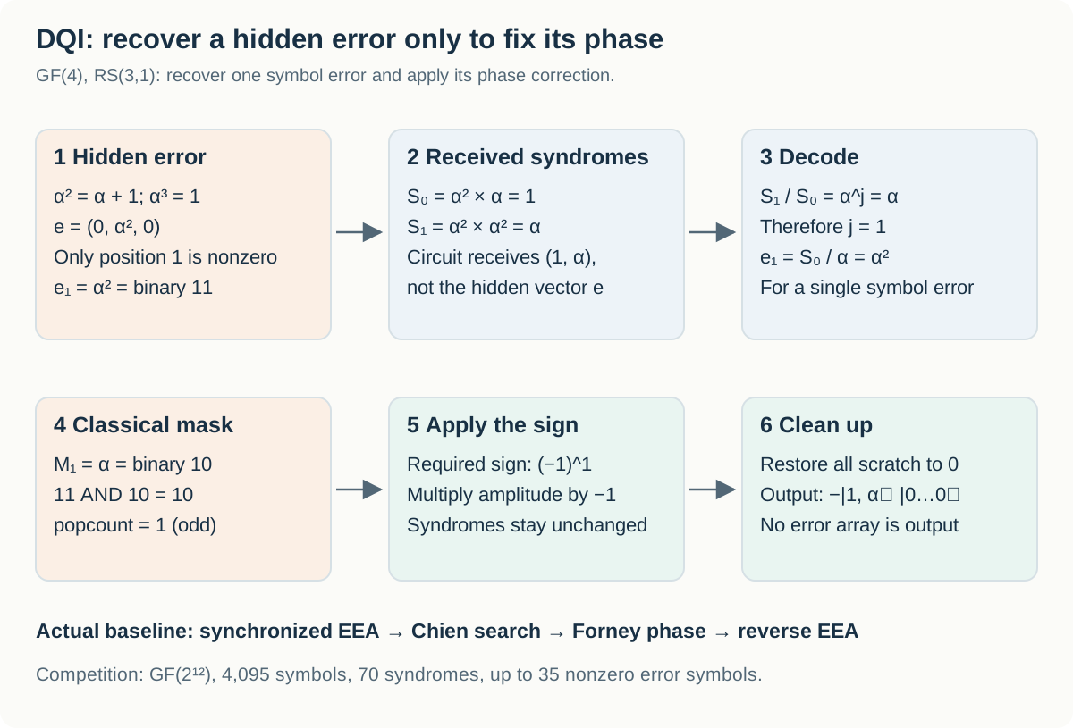
Figure 5. In this GF(4) teaching example, the received syndromes are $(1,\alpha)$. Decoding recovers the single error $e_1=\alpha^2$; the mask parity is odd, so the required sign is −1.
6.6. The reference circuit: EEA → Chien → Forney → uncomputation
For multiple errors, collect the syndromes into a polynomial:
\[S(z)=S_0+S_1z+\cdots+S_{69}z^{69}.\]If $J$ is the set of error positions, an error-locator polynomial $\sigma$ and an error-evaluator polynomial $\Omega$ satisfy
\[\sigma(z)=\prod_{j\in J}(1-\alpha^jz), \qquad \sigma(z)S(z)\equiv\Omega(z)\pmod{z^{70}}.\]In a field of characteristic 2, subtraction and addition are the same. The roots of $\sigma$ identify error locations; $\Omega$ helps recover their values. The congruence means that terms of degree 70 and above are discarded after multiplication.
| Stage | What it determines | What the official generator does |
|---|---|---|
| Solve the key equation | $\sigma,\Omega$ | A Proos–Zalka-style synchronized Extended Euclidean Algorithm (EEA), with 222 steps by default |
| Chien search | Which positions contain errors | Evaluates whether $\sigma(\alpha^{-j})=0$ at all 4,095 positions |
| Forney calculation and phase | Which sign the error value contributes | Uses $\Omega$, the inverse of $\sigma’$, and the mask to apply a phase product, then clears temporary values |
| Uncomputation | How to remove remaining quantum information | Reverses the EEA and initial alignment to restore the syndrome and zero the workspace |
With the simple normalization used above, an error location has $e_j=\Omega(\alpha^{-j})/\sigma’(\alpha^{-j})$. The official implementation folds exponent corrections for its EEA array representation into position-dependent constant multipliers. An implementation must therefore match the syndrome exponent convention and polynomial alignment, rather than copy a formula in isolation. In the GF(4) example, $\sigma(z)=1+\alpha z$, $\Omega(z)=1$, and $\sigma’(z)=\alpha$. At root $z=\alpha^2$, it recovers $1/\alpha=\alpha^2$.
The official generator’s forney_step constructs inversion workspace at each position, combines the error-location condition with $\Omega$, and calls gf2_phase_by_product(..., mask=...). It does not keep all 4,095 decoded error values in an array until the end. The reference circuit therefore already uses part of the idea of computing the phase without retaining complete values. A proposed improvement must identify what additional work or storage it eliminates.
6.7. Why a conventional CPU decoder cannot simply be inserted
A classical decoder can overwrite arrays, discard previous remainders, and stop a loop according to its data. A quantum circuit may receive a superposition of different syndromes. Applying those operations without a reversible construction can discard information or leave a record of the path taken. A reversible implementation must account for information needed to reconstruct earlier values, branch controls, and cleanup of temporary products.
CPU runtime alone is therefore not enough to choose an algorithm. This competition charges for Toffoli gates, including cleanup, qubits used, and failure rate under the official distribution. Recomputing an intermediate value may use more gates but less workspace; the $Q^2$ cost factor can make that a worthwhile trade.
The published reference uses 1,893 qubits and 5,725,461 Toffolis. Competition companion paper, Section III.2
6.8. A small failure rate is allowed, with a cost penalty
Official verification uses 102,400 shots. Each shot draws an error weight $w\in{0,\ldots,35}$, distinct error positions, nonzero error values, and measurement masks. Error weights are not uniform. To match the DQI state, the verifier constructs a 36×36 symmetric tridiagonal matrix and uses $\Pr[w]=v_w^2$, where $v$ is its normalized eigenvector for the largest eigenvalue:
\[A_{w,w}=\frac{w(q-2r)}{\sqrt{r(q-r)}},\qquad A_{w-1,w}=A_{w,w-1}=\sqrt{w(m-w+1)}, \quad(q,m,r)=(4096,4095,2016).\]Conditional on $w$, positions and nonzero values are sampled uniformly. The expected weight is approximately 31.05. Passing tests restricted to small numbers of errors does not establish correctness under the official distribution.
A changed syndrome or nonzero residual workspace counts as a value error. If the value checks pass but the sign is wrong, it counts as a phase error. The two categories are disjoint. For $k$ failed shots out of $N$, the cost uses the one-sided Clopper–Pearson upper bound $\epsilon_+$, rather than the empirical rate $k/N$:
\[\mathrm{cost}_{\mathrm{DQI}}=R(\epsilon_+)Q^2T, \qquad R(\epsilon)=\frac{\ln2}{-\ln(\tfrac12+2\sqrt\epsilon)}.\]The confidence level is $1-2^{-128}$; acceptance requires $\epsilon_+<1/16$. Here $T$ is the mean number of Toffoli-like gates actually executed per shot, including cleanup. The qubit count $Q$ includes the 840 input qubits and workspace. A circuit’s maximum static gate count can differ from its mean executed cost when gates are conditional.
Even with zero failures, $\epsilon_+=1-(2^{-128})^{1/102400}\approx0.00086606$ and $R\approx1.19126$. A finite sample is not treated as establishing an exactly zero failure probability.
| Hypothetical change | Cost ratio | Interpretation |
|---|---|---|
| 10% fewer qubits, unchanged Toffolis and $R$ | $0.9^2=0.81$ | 19% lower cost |
| 10% fewer qubits, 20% more Toffolis, unchanged $R$ | $0.9^2\times1.2=0.972$ | 2.8% lower cost |
| 10% fewer qubits, 30% more Toffolis, unchanged $R$ | $0.9^2\times1.3=1.053$ | 5.3% higher cost |
| 20% fewer Toffolis, 30% higher penalty $R$, unchanged qubits | $0.8\times1.3=1.04$ | 4% higher cost |
A shorter circuit with failures must remain cheaper after including the increase in $R$.
6.9. Where to begin optimizing
| Approach | Hypothesis to test | What must stay consistent | What to compare |
|---|---|---|---|
| Qubit lifetimes and reuse | Workspace that is not needed simultaneously can share qubits | Syndrome inputs and cleanup conditions at each point | Lower $Q$ against added computation in $Q^2T$ |
| Field multiplication and inversion | The same field operation can use fewer Toffolis or less workspace | Irreducible polynomial, bit basis, and convention for zero inputs | Cost of computation and cleanup together |
| EEA storage and addressing | Polynomial, remainder, or pointer storage can be reduced | The key equation and information needed for reversal | Whole-decoder $Q$ and $T$ |
| Chien and Forney stages | Per-position inversions or phase calculations can be shared or replaced | All 4,095 positions and the mask contract | Total repeated-stage cost and zeroed workspace |
| Another decoding algorithm | An alternative such as Berlekamp–Massey has a cheaper reversible realization | The same syndromes, field, masks, and distribution | Official cost and failure bound for the completed circuit |
Changing everything at once makes it difficult to locate a mistake in the field representation, position ordering, key equation, phase masks, or uncomputation. A useful progression is to check the mathematics on an exact small-field example, check one reversible primitive, and then expand to the official instance under the same contract. The completed circuit requires full official verification.
Primary sources for this task are the official data and verifier, the original DQI paper, the optimized reversible decoder paper, and Section III.2 of the competition companion paper.
Start with ProosAndZalkaDecoder in dqi_reference_circuit.py to follow initialization and forward/reverse EEA, then read the inverse, mask-phase, and cleanup logic in forney_step. Align build_reference_circuit with the verifier’s syndrome-exponent convention first.
7. dfthcsos: turning a molecular Hamiltonian into a smaller quantum program
7.1 Why does estimating molecular energy require expensive lookups?
The eventual chemistry application is to estimate a molecule’s ground-state energy: the lowest energy available to a system with a specified number of electrons. The competition task isolates a component of that calculation. Participants improve a compressed Hamiltonian representation and the circuits that load its data into a larger energy-estimation algorithm.
The Hamiltonian H describes how electrons move and interact. As with an ordinary matrix, its eigenvectors describe stationary states and its eigenvalues give their energies. Coefficients describing interactions between orbitals specify H without writing out the enormous matrix over every electronic configuration.
An orbital is a basis function for a single-particle state an electron can occupy. It does not mean one atom or a small box at a fixed location. Rather than assigning permanent labels to otherwise identical electrons, this representation describes the occupancy of allowed electronic modes. This is the second-quantized viewpoint used in this task.
The official instance, FeMoCo76o113e, concerns FeMoCo, the active center of the nitrogen-fixing enzyme nitrogenase. It uses 76 spatial orbitals and 113 electrons. Each spatial orbital has two spin modes. The number 76 therefore does not mean 76 electrons, 76 atoms, or a 76-qubit submission circuit. The baseline ANGLE circuit’s 119 qubits and the full cost model’s 730 qubits measure different resources again. These constants and the contract are documented in verifiers/dfthcsos/SCORING_README.md in the official competition data.
| Symbol | Meaning here | What the benchmark supplies |
|---|---|---|
| N | Number of spatial orbitals | 76 |
| η | Number of electrons | 113 |
| h⁽¹⁾ₚq | One-electron coefficients | Reference FCIDUMP coefficients with the prescribed transformation |
| h⁽²⁾ₚqrs | Two-electron interaction coefficients | A tensor indexed by four orbital indices |
| H | Hamiltonian of the full electronic system | The operator defined by those coefficients |
Intuitively, one-electron terms describe an electron’s motion and its interaction with its environment; two-electron terms describe interactions between electrons. Precise coefficient conventions depend on how creation and annihilation operators are ordered. The official implementation uses a consistent convention and transformation. The two-electron coefficients have four indices: p, q, r, and s.
If each index takes N values, a direct table has N⁴ entries. For N=76, that is 76⁴=33,362,176 entries. Symmetries remove redundancy, but translating every coefficient into costly branches in a quantum circuit is still unattractive. The starting idea is to compress the structure on a classical computer and build a smaller quantum program that reads and uses that structure.
7.2 Compress the numbers and the circuit together
Consider this small matrix:
\[A=\begin{pmatrix}1&2\\2&4\end{pmatrix} =\begin{pmatrix}1\\2\end{pmatrix} \begin{pmatrix}1&2\end{pmatrix} =5uu^{\mathsf T},\qquad u=\frac{1}{\sqrt5}\begin{pmatrix}1\\2\end{pmatrix}.\]Instead of storing four entries separately, we can reconstruct the matrix from a vector u and the weight 5. Real coefficient tensors are much larger and may not have an exact low-rank representation. A sum of a manageable number of simple components can still approximate them within an allowed error. This is the purpose of factorization.
The official dfthcsos task fixes a DFTHC factorization structure connecting double factorization and tensor hypercontraction, while allowing its dimensions and numerical parameters to change. The verifier reconstructs intermediate matrices using
It then adds outer products of these X matrices to reconstruct a four-index tensor:
\[G_{pqrs}=\sum_{\rho=1}^{R}\sum_{c=1}^{C} X^{(\rho c)}_{pq}X^{(\rho c)}_{rs}.\]The reference two-electron integrals are compared with G after undoing the prescribed symmetry-shift terms. G alone should therefore not be identified directly with the original integrals in all cases. The vectors u, weights w, identity offsets W, and fixed symmetry shift have distinct roles.
| Choice | Intuition | Tradeoff when reducing it |
|---|---|---|
| R | Number of outer factorization components | Fewer components may leave too little expressive capacity |
| B | Single-particle vectors per component | Fewer lookup addresses, but potentially larger reconstruction error |
| C | Coefficient copies per component | Both state-preparation cost and factorization flexibility change |
| u, w, W | Continuous numerical parameters | Equal reconstruction error can still give different normalization and circuit costs |
The factorization can be improved through numerical optimization, with the complete resource cost as its objective. At a given accuracy, a representation with fewer addresses, cheaper state preparation, and a smaller normalization multiplier can be better. It helps to feed the complete resource estimate back into the numerical choices rather than treating compression and circuit construction as independent jobs.
7.3 Block encoding: making the Hamiltonian usable inside a circuit
The reversible part of a quantum circuit must be unitary. A general Hamiltonian H is not unitary: multiplying a state by H does not necessarily preserve its length. We therefore cannot simply treat H as a gate.
Block encoding places a normalized operator inside a block of a larger unitary U. With an auxiliary register prepared in zero, the relevant block satisfies
\[(\langle0\rvert _{\mathrm{anc}}\otimes I)\, U\, (\lvert 0\rangle_{\mathrm{anc}}\otimes I) =\frac{\widetilde H}{\alpha}.\]Here H̃ is the Hamiltonian after any constant shifts or other transformations required by the algorithm, and α is a normalization that allows this block to fit inside a unitary. A larger energy-estimation algorithm repeatedly queries this operation and its inverse.
That repetition makes the implementation cost matter. Even a small reduction in one data lookup can help when it is called many times. A large normalization can also make it more expensive to resolve the desired energy differences. The benchmark therefore combines the cost of one block-encoding call with a normalization-related multiplier. Converting this resource cost into hardware runtime additionally requires a physical architecture and error-correction model.
DFTHC uses a sum-of-squares (SOS) structure after moving the energy reference: the shifted approximate Hamiltonian $H_{\mathrm{DFTHC}}-E_{\mathrm{SOS}}I$ is positive semidefinite on the fixed-electron-number sector. The square structure and shifted energy reference enable spectrum amplification. Two factorizations with similar approximation error can have different normalization costs and therefore different costs for the larger algorithm. The companion paper, Section III.3 and Appendix A, develops this connection.
The official verifier does not diagonalize the full many-electron Hamiltonian to obtain its ground state. It uses a fixed energy upper bound E_upper and the E_SOS calculated from the factorization:
\[E_{\mathrm{gap}}=E_{\mathrm{upper}}-E_{\mathrm{SOS}},\qquad \lambda_{\mathrm{eff}} =\sqrt{E_{\mathrm{gap}}(2\Lambda-E_{\mathrm{gap}})}.\]LCU (linear combination of unitaries) represents an operator as a weighted sum of unitaries. Λ is the raw normalization obtained from the coefficient magnitudes; the formula combines it with the SOS reference difference to obtain the effective multiplier λ_eff. In this formula, E_gap is the difference from the SOS reference; it is not the physical excitation gap between the ground state and first excited state. lambda_eff is an effective normalization multiplier in the score, rather than the molecule’s energy or its error.
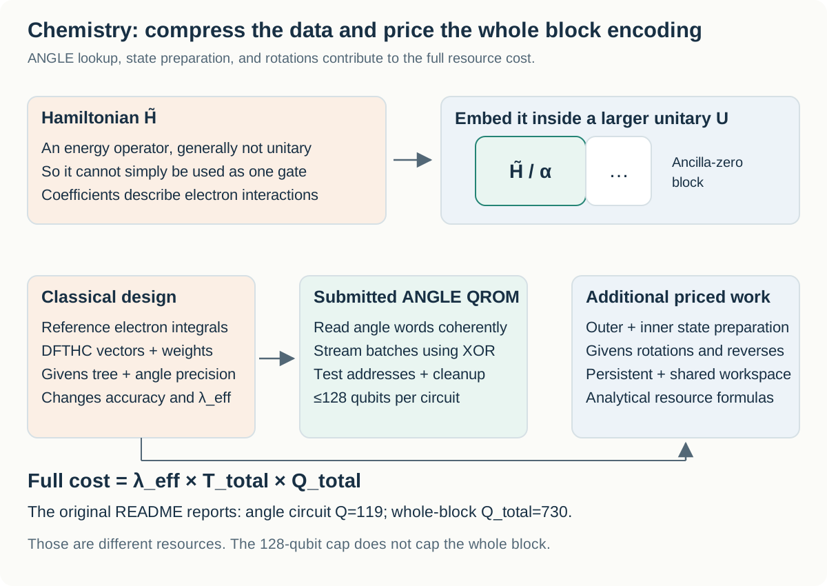
Figure 6. Coefficients lead to a factorization, a rotation tree, and ANGLE QROM circuits. The verifier simulates the angle-loading circuits, while state preparation and Givens rotations are priced analytically. Both branches contribute to the whole block-encoding score.
7.4 QROM: reading a table without measuring the address
In Python, table[a] reads row a. In a quantum algorithm, the address can be in a superposition. Measuring it to choose a single row would destroy that superposition. The lookup must instead preserve the address and reversibly XOR its corresponding data into a target register:
This is a QROM, or quantum read-only memory, lookup. It implements a known classical table as a gate pattern; it does not require a separate large quantum memory device. For a two-row table with d₀=01 and d₁=10, linearity gives
\[\frac{\lvert 0\rangle+\lvert 1\rangle}{\sqrt2}\lvert 00\rangle \longmapsto \frac{\lvert 0\rangle\lvert 01\rangle+\lvert 1\rangle\lvert 10\rangle}{\sqrt2}.\]Each address is now associated with its own data. The circuit has neither selected one row by measurement nor loaded an average of the rows. After the data have been used, applying the same XOR lookup again can clear the target back to zero. The competition also permits measurement-based uncomputation, provided the associated phase corrections are correct.
A lookup is not free array indexing in a quantum circuit. It requires reversible logic to select the address and gates to transfer the corresponding bits into the target. The number of addresses, output width, branching structure, and workspace-sharing schedule all affect the implementation.
7.5 Why represent vectors as tables of rotation angles?
Loading the components of a factorization vector u directly as quantum amplitudes is itself nontrivial. The official construction instead reads angles for a sequence of Givens rotations that represents u. A Givens rotation mixes just two components. The verifier recovers a vector from the angle table with the following 2×2 update; this is the coefficient-vector convention implemented by the verifier:
\[\begin{pmatrix}u_p'\\u_q'\end{pmatrix} =\begin{pmatrix}\cos\theta&-\sin\theta\\ \sin\theta&\cos\theta\end{pmatrix} \begin{pmatrix}u_p\\u_q\end{pmatrix}.\]For a three-component example, start with u=(1,0,0). Apply a π/4 rotation on the tree edge 0→1, then another π/4 rotation on 0→2:
\[(1,0,0) \xrightarrow{(0,1),\,\pi/4} (1/\sqrt2,1/\sqrt2,0) \xrightarrow{(0,2),\,\pi/4} (1/2,1/\sqrt2,1/2).\]Each step preserves length, so the final vector remains a unit vector. Changing the rotation-tree order can change the vector represented by the same angle values. The tree is consequently part of the submitted representation.
For N=76, one vector uses 75 tree edges and 75 angles. Those angles are finite-precision integer words rather than real numbers of unlimited precision. A b_rot-bit word means
\[\theta=\pi\frac{\mathrm{word}}{2^{b_{\mathrm{rot}}-1}}, \qquad 0\leq\mathrm{word}<2^{b_{\mathrm{rot}}}.\]The interval [0,2π) is therefore divided into a finite grid. At 12 bits, the grid spacing is 2π/4096 radians. Fewer bits can save angle-register space and rotation cost, but they also change the reconstructed vectors and coefficient tensors more. A high-precision factorization that meets the error limits may fail after its angles are rounded. The verifier evaluates the quantized angles actually loaded by the circuits.
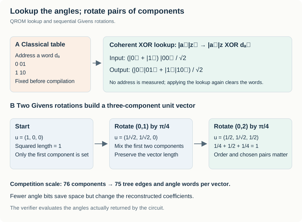
Figure 7. A two-address coherent QROM mapping and two successive two-mode Givens rotations.
7.6 Streaming 75 angles through a smaller register
Loading J angles at a time allows the same word registers to be reused. The baseline uses b_rot=12 and J=8, so the angle words occupy 96 qubits, and 75 angles are streamed in 10 batches. There are N+RB=76+65×60=3,976 vector addresses, requiring a 12-qubit address register.
Each ANGLE_k circuit does not first clear the current batch to zero and then write a new one. The contract loads the XOR difference between neighboring batches. For batches B₀,B₁,… at one address, define
If the register currently holds B₀, XORing δ₁ leaves B₁. The same word registers can thus carry data from one batch to the next. The final batch pads positions beyond the 75 angles with zeros, and reverse traversal must undo the sequence. Increasing J reduces the number of lookups, but it keeps more angle words alive at once and approaches the 128-qubit cap.
7.7 What is submitted, and what is actually checked?
| Component | Participant supplies | How it is assessed |
|---|---|---|
| Numerical factorization | Array shapes defining R,B,C, and weights | Reconstruction errors and normalization against the reference integrals |
| Rotation representation | tree_edges, word precision, and batch size | Unit vectors reconstructed from the angles recovered from the circuits |
| Angle loading | Circuits angle_k_0, …, angle_k_(K−1) | Every address, forward and reverse, with 64 shots per address |
| Remaining block-encoding operations | No complete implementation of these is submitted | State preparation and Givens rotations are priced with official analytical formulas |
The U array in submission.npz supplies its shape; the actual vectors are reconstructed from the angles loaded by the ANGLE circuits. Good vectors in the U array cannot substitute for a circuit that loads different angles. Submitted H1_I and Hsym_lower values are ignored, and the baseline’s fixed symmetry shift is used.
Every ANGLE circuit must preserve the address, return temporary qubits to zero, and leave no unwanted ±1 phase. Disagreement between repeated word samples, or a padding, reverse-traversal, phase, or workspace violation, causes rejection. The submitted circuit does not implement the Givens rotation itself with Z_POW: it is a Boolean oracle that loads binary angle words, and Z_POW is prohibited. The detailed contract is in the official data’s dfthcsos/SCORING_README.md.
7.8 The whole cost changes the optimization priorities
The official task cost is
\[C_{\mathrm{chem}}=\lambda_{\mathrm{eff}}\,T_{\mathrm{total}}\,Q_{\mathrm{total}}.\]Here T denotes a Toffoli count, not a count of T gates. The complete resource formulas are
\[T_{\mathrm{total}}= T_{\mathrm{ANGLE,fwd+rev}}+T_{\mathrm{outer}}+T_{\mathrm{inner}} +2(N-1)(2b_{\mathrm{rot}}-1),\]and
\[Q_{\mathrm{total}}= Q_{\mathrm{outer,persist}}+Q_{\mathrm{inner,persist}}+Jb_{\mathrm{rot}} +\max(Q_{\mathrm{outer,temp}},Q_{\mathrm{inner,temp}},Q_{\mathrm{ANGLE,temp}}).\]State preparation and angle lookup run sequentially, so temporary workspace is counted by its maximum, rather than its sum. Angle words remain live during the rotations, so their registers contribute to persistent space. Reducing the qubit count of one ANGLE circuit does not necessarily reduce total Q by the same amount.
| Official README baseline | Value |
|---|---|
| R,B,C / b_rot / J / number of batches K | 65,60,60 / 12 / 8 / 10 |
| One ANGLE circuit | 119 qubits; 3,974 Toffolis |
| Complete forward and reverse ANGLE traversal | 79,480 Toffolis |
| Outer preparation / inner preparation / Givens | 846 / 9,461 / 3,450 Toffolis |
| Total T_total | 93,237 |
| Total Q_total | 730 = 186 persistent + 544 shared temporary |
| Raw Λ / E_gap | Approximately 308.45594 / 3.96548 Ha |
| λ_eff / task cost | Approximately 49.30137 / 3.3556×10⁹ |
ANGLE lookups account for about 85% of baseline Toffolis. By contrast, much of the qubit cost comes from the 544 shared temporary qubits used by state preparation. Reducing lookup Toffolis and changing factorization dimensions or precision to reduce preparation space are therefore different opportunities. A lookup could even use more temporary qubits without increasing total Q, provided it stays below the existing temporary-space maximum and respects the 128-qubit ANGLE cap. The actual layout and official model must establish whether that room exists for a particular design.
Acceptance requires error_1 ≤ 20 mHa, error_2 ≤ 20 mHa, no ANGLE circuit above 128 qubits, Λ>49.0, E_gap>3.914898 Ha, and the valid domain 0<E_gap<2Λ. Equality at either strict Λ or E_gap floor is rejected. The two errors are Frobenius residuals of the reconstructed one-electron coefficients and two-electron coefficient tensor, respectively. These checks do not certify a many-electron ground-state energy error of at most 20 mHa.
7.9 How to approach a first improvement
| Approach | Keep fixed first | Change | Compare after acceptance |
|---|---|---|---|
| Improve the lookup circuit | Factorization, tree, and angle words | Address branching, shared logic, QROM construction | ANGLE Toffolis and temporary space for identical loaded words |
| Choose the batch size | Factorization, tree, and precision | J and the number of batches | The 128-qubit cap and total T and Q |
| Improve the tree and rounding | High-precision factorization | Tree and angle quantization | Reconstructed error_1, error_2, and λ_eff |
| Improve the factorization | Reference integrals, fixed shift, and final scoring formula | R,B,C and u,w,W | λ_eff×T_total×Q_total under the accuracy constraints |
Keeping the baseline angle table fixed while studying the QROM generator gives a relatively isolated first question. Changing the angle table at the same time makes circuit correctness, factorization quality, and rounding error move together. Someone with numerical-optimization experience may prefer to start with the high-precision factorization, but must still check reconstruction error at the eventual circuit precision.
Possible research directions include QROM constructions that spend more workspace to process groups of addresses, shared logic for repeated output bits, and joint choices of batches, trees, and rounding. Compare the complete cost after checking the official accuracy and resource constraints.
Read the worked example in SCORING_README.md → batch XOR tables in example_submission/angle_k_reference_circuit.py → evaluate_words in verify.py → vector and coefficient reconstruction in scoreinfra/dfthc_math.py. This separates reading the right words from making those words describe a good Hamiltonian.
8. Task cost and leaderboard score move in opposite directions
The three bottlenecks optimize different resource products.
| Task | Cost to reduce | What must stay fixed for comparison |
|---|---|---|
| invsqrt | Q×C, C=Toffolis+T gates/4 | Full x domain, phase error, synthesis margin |
| dqi | R(ε₊)×Q²×T | Field, syndromes, masks, official distribution |
| dfthcsos | λ_eff×T_total×Q_total | Reconstruction errors and whole-block resources |
In the latter two formulas, T is the Toffoli count, not T gates. For invsqrt, one arbitrary-angle rotation costs $0.56\log_2(1/\epsilon)+5.3$ T gates at synthesis error ε; C includes these synthesis costs.
Lower is better for each task’s cost. The final leaderboard score is the geometric mean of the improvements over the reference circuits, so higher is better:
\[\mathrm{Score} =\left(\prod_{b=1}^{3} \frac{\mathrm{cost}^{\mathrm{ref}}_b}{\mathrm{cost}_b} \right)^{1/3}.\]| Hypothetical change | Improvement factors across the three tasks | Overall score |
|---|---|---|
| Match the reference submission | 1, 1, 1 | 1.000 |
| Halve the cost of one task | 2, 1, 1 | About 1.260 |
| Reduce one task’s cost to one quarter | 4, 1, 1 | About 1.587 |
| Halve the cost of all three tasks | 2, 2, 2 | 2.000 |
A submission package must contain all three tasks. Use the official reference files for unchanged tasks.
The score field written by the invsqrt verifier is that task’s cost, Q×C: lower is better. The combined Kaggle score uses the geometric mean above.
9. The first files and environment to prepare
The official distribution contains circuits, verifiers, and numerical data instead of conventional train.csv and test.csv. The initial package contained 34 files totaling about 1.04 GB:
1
2
3
4
5
6
7
8
9
10
11
12
13
14
official/
├── sample_submission/
│   ├── invsqrt.kmb
│   ├── dqi.kmb
│   └── dfthcsos/
│       ├── angle_k_0.kmb ... angle_k_9.kmb
│       └── submission.npz
├── verifiers/
│   ├── invsqrt/
│   ├── dqi/
│   └── dfthcsos/
├── kickmix/
│   └── kickmix.so
└── verifiable_circuit_compilation.pdf
.kmx is a readable text circuit format; .kmb is binary. Both can be submitted. Python’s kickmix.Circuit and CircuitBuilder can read and generate circuits. To understand how numerical arrays and arithmetic become gates, start with the reference generator and builder API together rather than editing a circuit file directly.
Starting on Kaggle
For a path with less installation work, begin with the official starter notebook and data. Adding the supplied kickmix/ directory to Python’s search path allows the Kaggle distribution’s library to be imported. Check the notebook’s Input panel for the actual input mount path. Copying the same .so to a local machine with a different OS or Python ABI does not make it compatible.
On October 23, 2026, the data description listed a PyPI release of kickmix as planned. Use the supplied library or a source build until pip install kickmix is available for the target platform.
Local build configuration
The local reproduction used macOS arm64, Python 3.12.13, NumPy 2.2.6, and an Apple C++20 toolchain. Its standalone kickmix subpackage was built from this official Qualtran commit:
1
638777fac4379bc62e2a1e4a52cf1a1753895d48
Installation commands for those package versions require uv, Git, and a C++20 compiler for the platform:
1
2
3
4
5
6
mkdir quantum-circuit-start
cd quantum-circuit-start
uv venv --python 3.12.13
uv pip install --python .venv/bin/python 'numpy==2.2.6' \
  'kickmix @ git+https://github.com/quantumlib/Qualtran.git@638777fac4379bc62e2a1e4a52cf1a1753895d48#subdirectory=kickmix'
.venv/bin/python -I -c 'import numpy, kickmix; print(numpy.__version__); print(kickmix.__file__)'
Run all subsequent commands from quantum-circuit-start/ as well. Downloads require Kaggle CLI authentication and acceptance of the competition rules. Do not put API tokens in an article or repository. With the CLI already configured, the following downloads the original data and the separate metric notebook:
1
2
3
4
5
mkdir -p downloads official metric runs
kaggle competitions download google-verifiable-quantum-circuit-compilation -p downloads
.venv/bin/python -m zipfile -e \
  downloads/google-verifiable-quantum-circuit-compilation.zip official
kaggle kernels pull metric/google-quantum-ai-metric -p metric
Keep the official reference circuits and verifiers unmodified. Generate candidate circuits in a separate directory, and record SHA-256 hashes of the originals, candidates, and verifier files. The metric notebook also performs preflight checks on circuit loading, permitted gates, registers, and submission structure. Passing one task’s verifier script does not check the entire submission path.
The source commit used to build Kaggle’s supplied Linux binary is undisclosed. Parity between that binary and the local source build remains unconfirmed.
10. Running the invsqrt baseline to completion
Begin by checking a subset of inputs to confirm that paths and library loading work. The command below is a smoke run that retains the original 22-bit circuit and only reduces the range of x. It creates a new run directory; do not reuse a run name.
1
2
3
4
5
6
7
8
9
mkdir runs/invsqrt-smoke-001 && \
.venv/bin/python -I official/verifiers/invsqrt/verify_submission_invsqrt.py \
  official/sample_submission/invsqrt.kmb \
  --n-p 10 --beta 1 --precision-bits 24 --eta 218 \
  --max-x 64 --shots-per-x 64 \
  --batch-size 256 --max-workers 1 \
  --salt quantum-circuit-local-v1 \
  > runs/invsqrt-smoke-001/result.json \
  2> runs/invsqrt-smoke-001/stderr.log
The smoke profile uses 4,096 shots to check installation and the interface. Rotation-synthesis cost depends on the smallest error margin over the tested range, so it can differ from the full-profile cost.
For a full run, restore the upper bound of x to 3,133,452. The completed local run used the following arguments, with paths adapted to the directory layout above.
1
2
3
4
5
6
7
8
9
10
11
mkdir runs/invsqrt-full-001 && \
OMP_NUM_THREADS=1 OPENBLAS_NUM_THREADS=1 MKL_NUM_THREADS=1 \
VECLIB_MAXIMUM_THREADS=1 NUMEXPR_NUM_THREADS=1 \
.venv/bin/python -I official/verifiers/invsqrt/verify_submission_invsqrt.py \
  official/sample_submission/invsqrt.kmb \
  --n-p 10 --beta 1 --precision-bits 24 --eta 218 \
  --max-x 3133452 --shots-per-x 64 \
  --batch-size 256 --max-workers 4 \
  --salt quantum-circuit-local-v1 \
  > runs/invsqrt-full-001/result.json \
  2> runs/invsqrt-full-001/stderr.log
The command has no timeout of its own. The recorded local run used a separate parent process to impose a 1,800-second limit and record the start, finish, logs, and file hashes.
Because output goes to files, the terminal may remain quiet during execution. Once the command finishes, open the result:
1
.venv/bin/python -m json.tool runs/invsqrt-full-001/result.json
Check that the process completed successfully, status is PASS, and verified_shots is 200,540,928. Compare num_qubits and score with the table below. For FAIL, read the JSON’s error and stderr.log. This JSON has no elapsed-time field. The 199.921 seconds below was measured separately by the parent process and stored in the run receipt.
The measured result
The full local run of the unmodified sample_submission/invsqrt.kmb produced these results. The runtime is a measurement from one execution.
| Measurement | Result |
|---|---|
| Verification status | PASS |
| Shots checked | 200,540,928 |
| Qubit count Q | 260 |
| Toffoli count per shot | 7,735 |
| Directly counted T gates | 1 |
| Arbitrary-angle rotations charged for synthesis | 37 |
| Toffoli-equivalent C, including synthesis | 7,987.593206597238 |
| Task cost Q×C | 2,076,774.233715282 |
| Verification-process wall time | 199.921 seconds, about 3 minutes 20 seconds |
| Verification workers | 4 |
The JSON field t_count: 1 does not mean rotation cost is negligible. Synthesis costs for the 37 rotations enter the final toffoli_equivalent. The largest ratio of phase error to allowed tolerance was approximately 0.476912, at x=2,588,411. Any precision reduction changes that margin and requires another full check.
The SHA-256 hash of the original circuit identifies the reproduction target:
1
e2bf8eb64350a4460a271fc7f1d591ef125b1e276377e9a0f64b96ab3ca321e1
The measured time includes Python process startup, circuit loading, and verification, and excludes preflight file hashing. It is the runtime of the local classical verifier, not the hardware execution time of the quantum circuit. Its scope and environment also differ from the approximately 45 minutes quoted in the official overview for scoring a full submission.
11. A minimal structure for continuing the experiments
Separate official originals, candidate-generation code, and run results so each comparison can be reproduced:
1
2
3
4
5
6
7
8
9
project/
├── AGENTS.md / CLAUDE.md        # Shared entry instructions and tool-specific routing
├── TODO.md / DECISIONS.md      # Next work / decisions with supporting evidence
├── docs/                      # Intent, policy, and resource guide
├── .agents/skills/             # Reusable execution procedures
├── .agent_runtime/exchange/    # Dated review requests and replies
├── data/official/<snapshot>/   # Unmodified official originals and manifest
├── candidates/                # Generation code and candidates, added when needed
└── runs/<run-id>/              # Results, logs, and receipt for one execution
Add candidate generators under candidates/ as experiments require them.
The essential record of a run is straightforward: which original and candidate were run, with which code, environment, randomness, and resource limits; whether verification finished and passed; and what it cost in resources and time. Preserve failed and interrupted attempts too. This keeps an incomplete run with an apparently low cost from being presented alongside a successful candidate as an improvement.
Claude and Codex reviews are recorded in dated exchange documents. Proposals and acceptance or revision comments accumulate there, while DECISIONS.md owns settled choices, TODO.md owns current work, and run receipts own measurements.
12. Submission format and dates to check
The following files belong at the top level of the submission ZIP:
1
2
3
4
5
6
7
8
submission.zip
├── invsqrt.kmb                 # Or .kmx
├── dqi.kmb                     # Or .kmx
└── dfthcsos/
    ├── angle_k_0.kmb
    ├── angle_k_1.kmb
    ├── ...                    # Consecutive numbering from 0, with no gaps
    └── submission.npz
submission.npz contains U, W, H2_I, H1_I, Hsym_lower, and tree_edges. Generating circuit files alone does not make a submission ready. The full metric’s preflight checks, each task’s verification, ZIP paths, and required files must also be checked. The official evaluation page documents the file contract.
Deadlines are at 23:59 UTC on the listed day, or 08:59 the next day in Korea.
| UTC date | Event |
|---|---|
| 2026-10-22 | Competition begins |
| 2026-11-20 | Intermediate milestone prize cutoff |
| 2027-01-04 | End of Longest Leader accumulation and its public-material deadline |
| 2027-01-13 | Rules-acceptance and team-merger deadline |
| 2027-01-20 | Final submission deadline |
The total prize pool is $150,000. Teams may have up to 5 members, with at most 5 submissions per day and 2 final selections. The intermediate, longest-leader, and task-specific additional prizes have separate requirements, including public materials; consult the prize description and rules.
Start with the official originals, run the invsqrt baseline, and confirm its PASS and cost. Then change one mechanism and compare it under the same verification conditions.
13. How the competition may develop
In Santa 2023, competitors designed moves around the mathematical structure of the puzzles and used cancellations between move sequences to shorten solutions. In Santa 2024, a lightweight neural network screened word permutations before expensive Gemma scoring. Santa 2023 released solution · Santa 2024 released solution
Here, the same proportional improvement contributes equally whichever task it comes from: the overall score is the geometric mean of the three improvement ratios. With the other two costs held constant, halving any task’s cost multiplies the overall score by $2^{1/3}$. Each task also has a separate USD 10,000 performance prize, giving both single-task specialists and teams dividing the three tasks a reason to participate. Official prizes
Reducing Toffolis alone is insufficient. DQI is particularly sensitive to qubit count because its cost includes Q². At the same failure-rate bound, halving the Toffoli count while increasing the qubit count by a factor of $\sqrt{2}$ leaves the cost unchanged. Designs that retain less intermediate state and uncompute cheaply may therefore matter more than a direct translation of a fast classical decoder.
Adapting released circuits to the competition could produce large early gains. Gu et al. replaced DQI’s EEA with Berlekamp–Massey and reduced the intermediate storage needed for uncomputation. The released implementation must be adapted to the competition’s interface and cost model and checked with its official verifier. Later progress may combine refinements to these implementations with new approximations, decoders, factorizations, and QROM designs.
Public-notebook requirements for milestone and longest-leader awards create an incentive to share improvements during the competition; the longest-leader award has its own publication deadline. Toward the end, implementation quality and adequate margins for phase error and DQI failure rates are likely to become increasingly important. Public and Private check the same submitted circuit using different salts and measurement outcomes. A circuit that survives those different checks should be a stronger final choice than one supported by a single favorable run. Official prizes · Evaluation · Metric implementation
References
- Kaggle competition · Evaluation · Data · Domain context · Timeline · Rules
- Official Google Quantum AI Metric — implementation of submission loading, preflight checks, and the combined three-task score.
- Khattar et al., Leveraging verifiable structure in quantum circuits to find more efficient compilations with agentic AI — the competition’s companion paper.
- Qualtran kickmix documentation · Source commit used for this local build
- DFTHC starter kit · Starter notebook
- Gu et al., Discovering state-of-the-art quantum circuits with large language models · Implementation repository
- Kaggle CLI — downloads and authentication setup.