RSNA Knee, Part 4: Conflicting Evidence and Two Final Candidates

Select a figure to enlarge it. On small screens, wide tables and equations scroll horizontally.

My current final selections are v229 at 0.957 and v236 at 0.953. The public Helios prediction, H, scores higher at 0.958, and a clean composition close to my second choice has scored 0.954. I have selected the pair despite those stronger Public alternatives because the local evaluations and Public favor different candidates.

The two submissions are separate candidates, not ingredients for another average. The second helps only if it outperforms the first on Private. A different architecture or lower prediction correlation does not establish that it will. I need to consider the actual differences and the unfavorable evidence that comes with choosing them.

It is October 22, 2026, at 09:00 KST (00:00 UTC). The deadline is October 22 at 23:59 UTC, or October 23 at 08:59 in Korea. I do not yet know the Private scores or my final rank.

Uses of public assets

In this final week, strong public predictions have become an alternative to training another model. Available systems include CoAtNet with mixed supervision and auxiliary data, compact ConvNeXt inputs with finding-specific pooling, and rank or probability blends with finding-specific weights. Their reported gains cannot be added together. Several notebooks reuse the same checkpoints, and apparently different combinations can share much of their prediction content.

I distinguish three uses of public material. A ready checkpoint can enter test inference without supplying compatible OOF. Retraining a complete recipe on my folds can produce a clean family for comparison with other models. Importing an input or pooling idea allows a controlled test of that component. These serve different purposes: testing a complete predictor, building reusable held-out predictions, and investigating a mechanism. Treating them alike would either exclude useful public predictions or misclassify full-data predictions as clean OOF.

The leaderboard also affects how I use public material. In the snapshot I saved yesterday, October 21, 1,471 of 6,307 teams displayed 0.958. Another 228 teams scored higher, placing the 0.958 group at ranks 229 through 1,699. With so many teams at that level, reproducing it is only part of the task; I also need to consider what I can add.

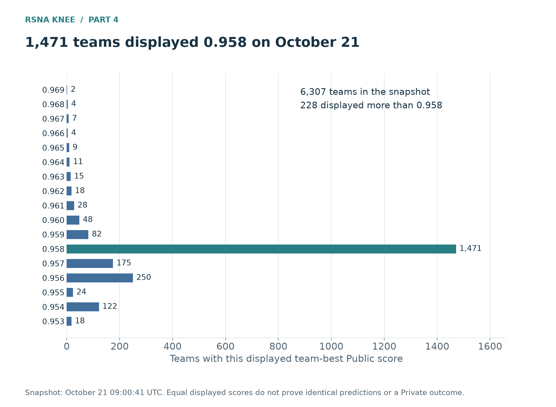Figure 1. Team-best Public scores at or above 0.953, from the October 21 09:00:41 UTC snapshot. The large 0.958 group describes score density. It does not prove identical prediction vectors, identify every team’s model ancestry, or assign a hypothetical final rank to an individual submission.

Reproducing a public prediction provides a strong benchmark, but the same predictions on the same studies cannot distinguish a copy from its original. A matching three-decimal score does not prove a copy, either: different unrounded AUCs or prediction vectors can share that display. I cannot infer that all 1,471 teams used identical predictions, or that they will move together on Private.

Several final choices remain possible. I can keep H with its Public advantage, blend it with my predictions, or retain a clean composition. Choosing a different composition makes sense if its differences improve rankings on unseen studies. Being self-trained or having clean OOF is not itself a test-score gain. Nor does a crowded Public score establish that H will be weak on Private.

I have used that distinction to choose the remaining experiments. I reproduce a public recipe when I can finish training and inference preparation and expect a useful new family. For a blend, I first specify the change and how its result could affect the final selection. Repeated small weight adjustments around a popular combination would make it harder to tell whether my predictions contribute useful information.

Label results and new model families

When I wrote Part 3 on October 15, N’s multimodal-label comparison was still incomplete. Later that day, N-mm12 scored 0.945 on Public against 0.942 for its definition-guided version. The locally favorable target change also improved Public in the full-field model. I included N-mm12 among the candidates for subsequent ensembles.

Two complete reproductions of public recipes expanded the clean comparison further. R949F, a CoAtNet recipe with the donor’s preprocessing, continuous mixed supervision, and auxiliary OAI data, scored 0.944 on October 16. The related earlier submission used for comparison had scored 0.937. S6F, a ConvNeXt-S recipe with finding-specific spatial and window attention, scored 0.952 on October 17. Both produced complete image-held-out OOF, retaining the source-label exposure to expert cases described in Part 3. S6F also strengthened the evaluated whole-bank selection procedure under the declared runtime budgets.

These results supported reproducing a coherent learning system when its components plausibly worked together. Input geometry determines what the encoder sees; the attention head determines which features contribute to each finding; supervision determines the distinctions those features learn. Changing all three means that the observed improvement cannot be assigned to the backbone alone. It can nevertheless establish a stronger model family to combine with independently trained alternatives.

Teacher supervision produced a different kind of candidate. N-T* scored 0.951 on October 16. Its targets included predictions whose ancestry did not preserve the exclusions needed for clean student OOF, so I treated it as final-only. Combining the full-field and 2.5D-window T* students scored 0.950, below N-T* alone. Two successful students did not imply an improved average: their common teacher content could reinforce similar rankings while their remaining differences hurt useful positive–negative pairs.

I use two kinds of evidence when selecting predictions. For clean models, I compare combinations on the same held-out studies and evaluate the selection procedure across folds. A complete mixture containing public or teacher-derived predictions cannot be assessed that way, so it needs a separate test comparison. This distinction identifies the evidence behind a choice rather than prohibiting a useful predictor.

The final pair: compositions and operators

My first selected candidate, v229, is dominated by the public Helios prediction H. My contribution is a block containing the five fold models of N-mm12 and five of V3-mm12, the 80-slice model. Write $R$ for a per-finding percentile-rank transformation. I average the ten members’ individual ranks and then form the outer blend:

\[\begin{aligned} A_{10}&=\frac{1}{10}\sum_{m=1}^{10}R(p_m),\\ C2_{0.25}&=0.75\,R(H)+0.25\,R(A_{10}). \end{aligned}\]

Ranking before averaging prevents one member’s probability scale from dominating simply because its predictions are more spread out. It does not make all aggregation orders equivalent. Ranking a family’s probability mean and averaging the ranks of its members can produce different study orders. The extra outer rank also converts the own block’s aggregated values back to a common scale beside H.

The complete v229 mixture is final-only because H lacks compatible clean OOF. Its N/V3 constituents retain their clean status. I can study those held-out predictions, but their evaluation does not validate the H-dominated final mixture.

My second selected candidate, v236, is K-W2, a probability combination of three clean families:

\[\begin{aligned} K\text{-}W2&=0.50\,B_{10}+0.25\,N+0.25\,V3,\\ B_q&=\sigma\!\left(\frac{1}{q}\sum_{m=1}^{q}z_m\right). \end{aligned}\]

Here $z_m$ is an S6F checkpoint’s logit. $B_{10}$ combines two seeds across five folds each. N and V3 are their respective five-fold probability means. The earlier K-W, v231, used $B_5$ with the same outer weights. Adding an S6F seed changed the estimate inside a family while leaving its final weight at one half. These expressions describe hidden inference. For a local OOF study, I use only the held-out checkpoint from each seed, comparing $q=1$ with $q=2$ inside the S6F block.

This nesting is important. Sigmoid of mean logits is not mean probability; averaging twenty checkpoint predictions with equal weights would also give a different answer. A checkpoint count describes computational work, not its final vote. These exact operators define what the comparison between K-W and K-W2 can tell me.

Comparison	v229	v236, K-W2
Public	0.957	0.953
Composition	H 0.75 + N/V3 rank block 0.25	S6F two-seed block 0.50 + N 0.25 + V3 0.25
Local evaluation	Whole mixture final-only	Complete clean OOF for the constituent families
Close alternative	v227, own share 0.50, Public 0.956	v231, one S6F seed, Public 0.954

My current pair consists of an H-dominated rank blend and an S6F-heavy clean probability blend. Both contain N and V3, so the different construction does not make them independent.

Longer training versus additional seeds

A promising ensemble did not settle what to train next. S6F was already the strongest clean family on Public, but its 16-epoch recipe left a plausible question: would a larger training budget improve it further? Another seed asked a different question. It repeated a working learning recipe to change the estimate obtained from its finite training process, rather than trying to learn a stronger representation with a longer schedule.

I tested the longer-budget hypothesis with a fresh 32-epoch S6F pilot. This stretched the cosine and warmup schedule from initialization; it did not continue the 16-epoch checkpoint for sixteen more epochs. The planned complete five-fold cost was about 18.5 GPU-hours, of which about 3.7 belonged to the first fold and 14.8 remained afterward. These were reserved training hours on the cached single-GPU machine, not the nine-hour hidden-inference allowance.

The pilot provided a particularly useful distinction between standalone quality and ensemble contribution. On 870 matched non-gold studies, the result was:

Fold-0 replacement, e32 minus e16	Primary difference	Saved report-group interval
S6F alone	−0.00622	[−0.01117, −0.00140]
S6F replaced inside fixed K-W	+0.00062	[−0.00165, +0.00267]

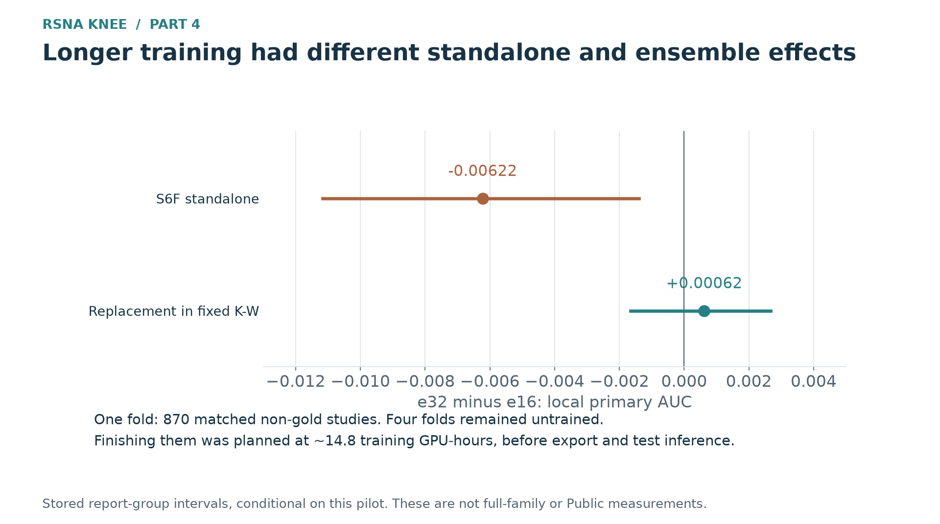Figure 2. The longer S6F recipe deteriorated alone while its fixed K-W replacement remained uncertain. Both contrasts use the same 870 matched fold-0 studies. The intervals describe conditional report-group variation; the remaining four folds were not trained.

Nine of twelve standalone finding scores fell. Yet replacing S6F inside K-W produced a small positive point estimate with an interval spanning zero. A weaker standalone prediction can change the difficult pairwise orderings of an existing ensemble differently from those it gets wrong alone. The pilot therefore did not justify the easy conclusion that a lower standalone score meant no possible ensemble value.

The difficult decision concerned what information the remaining 14.8 planned hours would buy. Completing the family could reveal whether fold 0 misrepresented the longer recipe and whether the full ensemble benefited. It would also delay the multimodal-label S6F variant and another seed of the established recipe by roughly fifteen hours. Their checkpoints still needed export, evaluation, and a complete test prediction before they could affect the final choice. A training result arriving just before the deadline would not have the same practical value as one I could actually compare.

I stopped the e32 pilot after weighing those alternatives. The uncertain K-W benefit, the standalone and target deterioration, and the alternative uses of the same machine together favored that choice. The partial predictions and checkpoint remained available, but there was no completed e32 family or Public result. Stopping gave up the full-family answer; it did not establish that S6F had converged or that every longer schedule would fail.

The existing two-seed S6F evidence helped make the alternative credible, but was not a calibrated return-per-hour comparison. Its approximately +0.000945 inside K-W came from complete OOF, whereas the e32 estimate came from one fold. Dividing those values by training hours would hide the different experiments. The choice was to prioritize a working recipe with positive complete evidence while preserving the unresolved longer-training idea, rather than to turn a pilot into a universal early-stopping rule.

OOF composition selection and inference readiness

A separate question was whether the accumulated families could already produce substantially more than the compact K-W prediction. Restricting every experiment to adding one model to the current reference could miss a better replacement or a different combination. I therefore used whole-bank searches that could add, remove, and replace families. The reference remained a comparison, not compulsory membership.

The October 19 search compared two conditions on 4,349 non-gold studies. P540 used one S6F seed and a 540-minute planning ceiling. PUNC used the two-seed S6F prediction and effectively removed the ceiling. Both optimized the Opus/GPT primary over 146 families with probability aggregation, a beam width of 16, at most ten rounds, and at most 50,000 sets per outer fold. They were substantial bounded searches, not exhaustive optimization over every ensemble operator and weight.

The distinction between a selected procedure and one final fixed composition matters here. For fold $k$, the selector chose a composition using the other folds and evaluated it on $k$:

\[S_{-k}=\operatorname{Select}(D_{-k}), \qquad \widehat A_{\mathrm{select}}=\frac1K\sum_k A_r(D_k,p_{S_{-k}}).\]

Fitting one composition on all the data gives another object, $S_{\mathrm{all}}$. Its score on the data used to choose it cannot simply inherit the procedure’s held-out estimate. In this study, a smaller procedure that picked the best fourth family chose different GPT-label models across folds. I then fixed one additional family, $U$, and combined it as $C1U=0.8\,K\text{-}W+0.2\,U$. C1U was this four-family prediction, not the added family alone. Its post-selection score was not a new untouched validation of that winner.

Comparison on the same studies and primary	Pooled AUC	Mean within-fold AUC
Fixed K-W	0.901375	0.901405
Best-fourth-family selection procedure	0.902831	0.902951
P540 c1 procedure	0.902772	0.903094
PUNC c1 procedure	0.902750	0.903067
Fixed C1U, selected after the scan	0.903310	0.903372

The large searches did not show a compelling extra primary payoff over the small fourth-family procedure. Their fitted delivery proposals were much heavier: seven families at 535.3 planning minutes for P540, and eleven at 1009.7 for PUNC. The near-cap P540 alternative also introduced decoding groups and little nominal margin. Similar conditional scores did not make these proposals equally ready to execute.

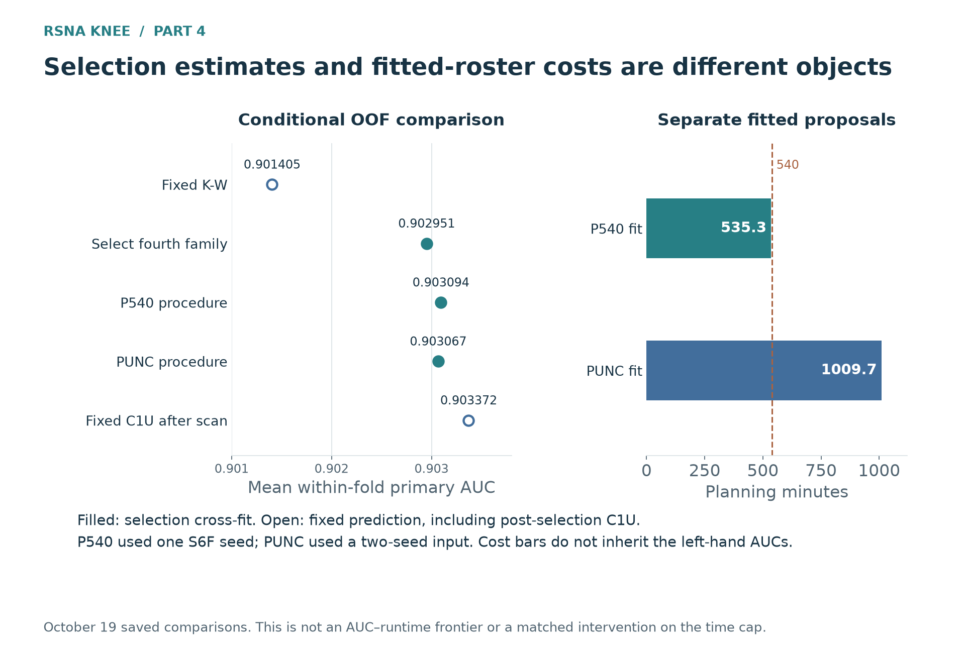Figure 3. Selection-procedure scores and fitted-proposal planning times answer different questions. P540 and PUNC also use different S6F inputs, so their score difference does not isolate the effect of removing the time ceiling. The fitted rosters do not inherit the procedure estimates as their own validated AUCs.

These results do not establish that the runtime cap has no effect on performance. It changed the selected composition and cost, while the uncapped condition also changed S6F content. This search found no useful additional primary point gain from its larger compositions. A different objective, aggregation operator or search could behave differently. That is a reason to defer one expensive implementation, not to declare the OOF bank exhausted.

C1U also changed direction with the evaluation labels. Opus gave about +0.001910 and DeepSeek +0.001773, while Gemini3f gave −0.001235 and dread −0.001779. All twelve findings deteriorated under dread. These are opposing assessments of the same predictions, not independent votes. Primary also includes the GPT source used to train the added family. I cannot select the largest favorable number and ignore the contrary results.

The OOF bank has already informed many choices. Selection cross-fitting did not retrain every base model inside each outer split, and the saved bootstrap intervals do not include all recipe, seed and candidate-selection variation. Given those limits, I chose one fixed C1U Public comparison with K-W still available, rather than immediately implementing a near-cap composition.

The subsequent 155-family refresh raised a similar issue. New seeds changed the recommended composition, but its fitted 533.8-minute roster still needs assembly and execution checks. Three equally weighted probability groups give S6F three fifths of the total; replacing them with one logit-averaged bundle would change the prediction. Mixed fold and finding results do not justify running it before the ready comparisons. More complete families expand the combinations I can study, but need not enter every final prediction.

Public scores and blend-weight comparisons

The equal-family combination of S6F, N-mm12 and V3-mm12 scored 0.953. Increasing S6F’s probability weight to one half produced K-W at 0.954. In this comparison, emphasizing the stronger S6F family worked better than weighting the three families equally.

I also compared the share of my predictions beside H. An own share of 0.50 gave v227 at 0.956; a share of 0.25 gave v229 at 0.957; H alone scored 0.958. Increasing the own share lowered Public. These results did not show an improvement over H from adding my predictions.

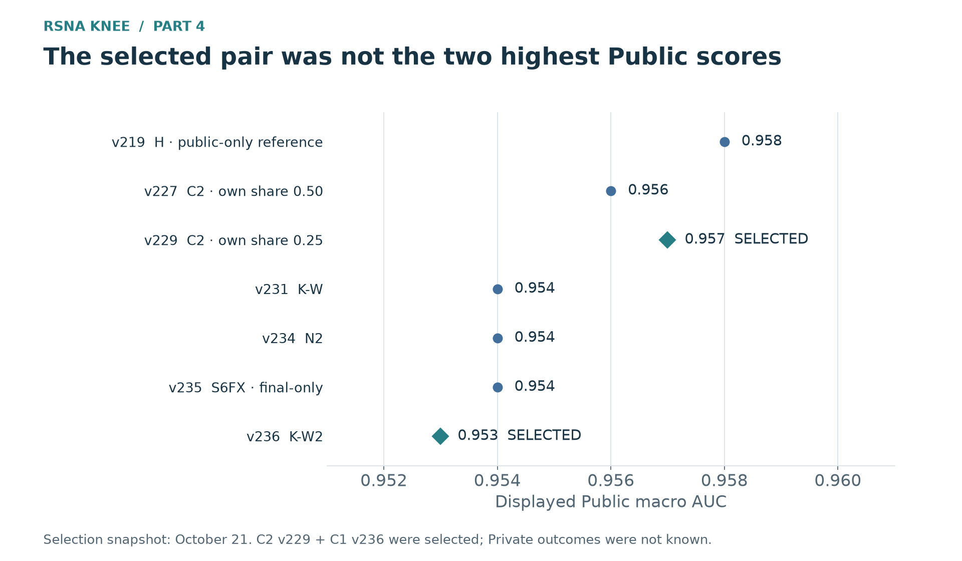Figure 4. Completed Public comparisons, including H, the selected v229 and v236, and their scored alternatives. A timeout supplies no AUC and is not represented as a low-quality prediction.

Because clean OOF cannot evaluate the complete mixture, I compared a few substantially different weights on Public. Filling the gaps with repeated small steps would increasingly select weights for the same exposed Public studies. I slightly prefer 0.25 to 0.50, but the displayed difference does not identify an optimum. H alone remains a strong option if I prioritize the highest Public score.

The clean variants tested content as well as allocation:

Candidate	Change relative to K-W	Public
C1U, v233	Additional GPT-label family and changed allocation	0.951
N2, v234	Two N seeds, with changed content and allocation	0.954
S6FX, v235	Full-data model inside the S6F block; final-only	0.954
K-W2, v236	Two S6F seeds, keeping the family weights	0.953

C1U did not reproduce its expected OOF improvement on Public. I preserved the added family’s clean predictions for other combinations. N2’s equal Public score does not establish that another seed had no effect, because the N/V3 allocation also changed. S6FX includes a full-data model: it can contribute to final inference, but the whole mixture cannot be treated as clean local validation. K-W2 keeps N, V3 and the outer weights fixed, making it the closest comparison of the added S6F seed.

Where model content and weights changed together, the result cannot be attributed to one of them alone. Acquiring another family is not a reason to put every family into a larger final composition.

Local and Public evaluations of K-W2

K-W2 improved the matched clean primary score over K-W by approximately 0.00095. The saved conditional interval was about +0.00055 to +0.00136. All five fold differences were positive, as were the other evaluated valid report-label readers, although four findings had small losses. Public moved in the opposite direction: 0.953 instead of 0.954.

I give the K-W2 local result weight because it holds the other predictions fixed. Only S6F changes from one seed to two, and the gain is not concentrated in one fold. Several reference-label evaluations improve, but they share reports and related assumptions. This is consistent improvement on the observed studies, not several independent expert validations.

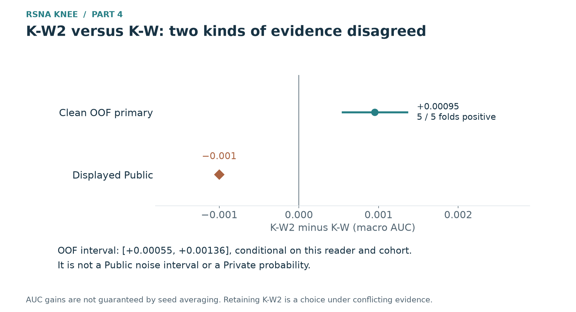Figure 5. K-W2 minus K-W: the local primary difference is about +0.00095, with its saved conditional interval, while displayed Public changes by −0.001. The interval concerns the local comparison; it does not measure Public noise or the probability of a Private reversal.

Why could another seed help locally and hurt elsewhere? For a probability blend, with $m$ indexing its probability components, the margin on a positive–negative pair is

\[D_{ab}=\sum_m w_m\bigl[p_m(x_a^+)-p_m(x_b^-)\bigr].\]

AUC counts whether these margins are positive, with half-credit for ties. An added prediction can reinforce a correct ordering, repair a wrong one, or reverse a narrow correct margin. Reducing prediction variability is not the same objective as improving every relevant ordering. S6F’s inner logit average changes the calculation, but the same pairwise issue remains: the studies near a ranking boundary matter more than agreement on easy pairs.

This is also why overall prediction correlation is insufficient. Two models can correlate closely across thousands of easy cases and disagree on the relatively few pairs that determine the AUC difference. A new reference changes which studies count as positive; a new test distribution changes which difficult examples occur. The relative usefulness of a seed can therefore change without either observed result being fictitious.

Execution limits of larger ensembles

I also tested larger compositions of the models already trained. These combined two S6F seeds with a second N seed, expanded S6F to three seeds, or placed the full-data model X inside S6F’s logit average. Each changed different models or weights and needed a separate comparison.

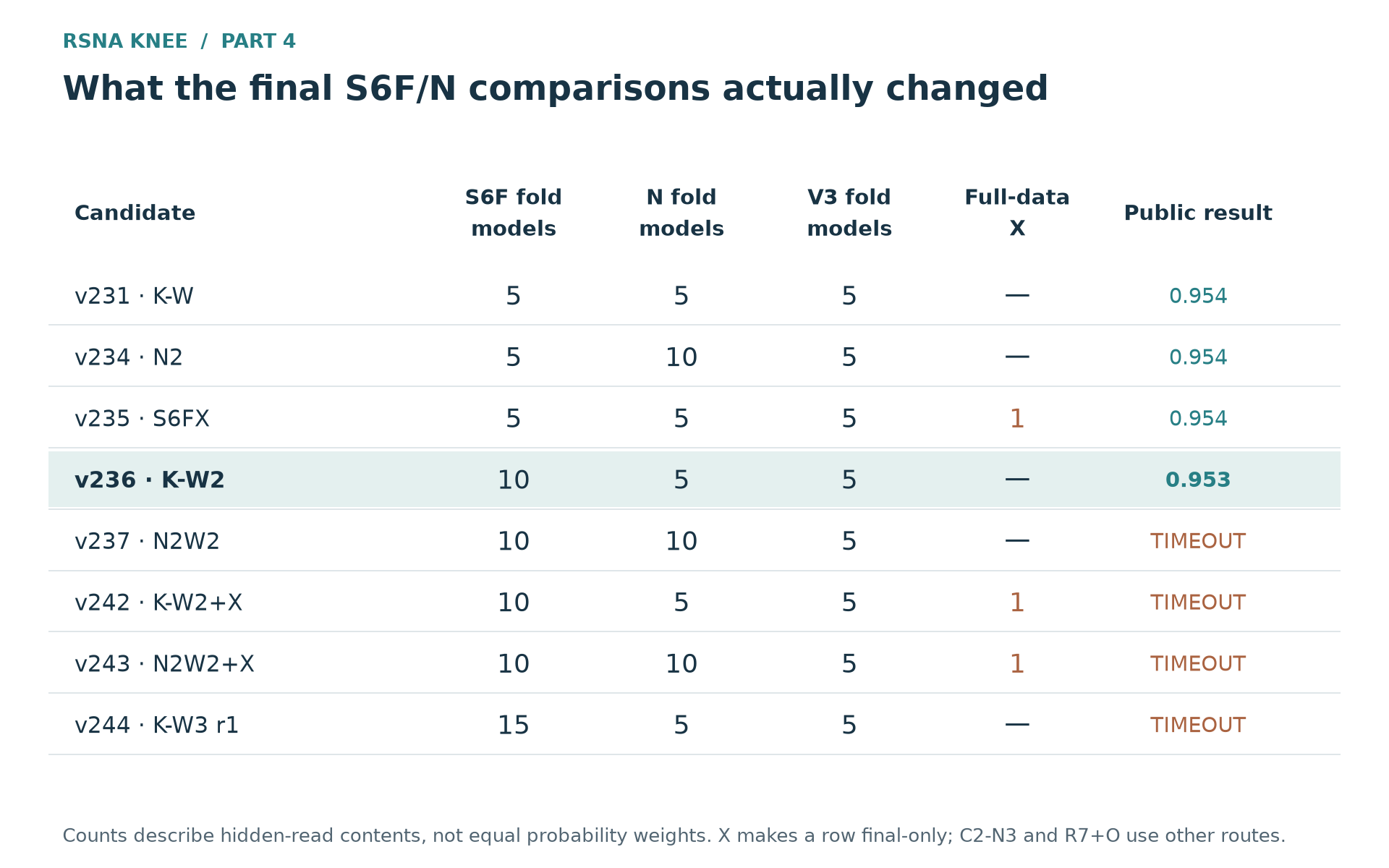Figure 6. Fold-checkpoint counts for related S6F, N, and V3 combinations, with X separately identified as a full-data model. Counts are not final probability weights. S6F retains an outer weight of 0.5, and X makes its descendants final-only. C2-N3 and R7+O use different constructions.

N2W2 combined two S6F seeds with two N seeds, changing N/V3 allocation as well as model content. K-W3 added a third S6F seed at the same outer weight. In S6FX, X was one of six S6 models; in K-W2+X, it was one of eleven. A favorable result for the former would not predict the latter’s contribution, because X’s weight inside the block changed. C2-N3 instead enlarged v229’s own rank block from ten to fifteen members at a fixed outer share.

All six larger complete-or-fail trials ended without a score:

Candidate	Question	Result
v237, N2W2	Two S6F seeds together with two N seeds	Timeout; no AUC
v238, C2-N3	Fifteen-model own rank block beside H	Timeout; no AUC
v240, R7+O	Public R7 with a larger final-only own block	Timeout; no AUC
v242, K-W2+X	Full-data X inside the two-seed S6F block	Timeout; no AUC
v243, N2W2+X	X inside the larger S6F/N combination	Timeout; no AUC
v244 retry 1, K-W3	Third S6F seed at the same family weight	Timeout; no AUC

The original v244 attempt ended in a platform system error; its retry timed out. I can establish that the submitted implementation did not finish within the permitted execution time, not that the model idea had a low AUC. I also lack enough hidden-stage timing detail to identify the failing stage or the extra time it would have needed.

Planning time alone cannot guarantee completion. Shared image decoding and two-GPU scheduling make total runtime differ from a sum of separate runs. More models can also change memory use and scheduling. Success for one composition and failure for a slightly larger one do not define a universal safe boundary. I can select the successful candidates; these six are not yet available for selection.

Before the deadline, I need time to inspect a result as well as produce it. Preparation, full inference, platform waiting and collection must all finish before a prediction can change the final selection. Without an implementation change or new execution evidence, repeating a timeout only uses another remaining opportunity. For now, I am keeping the scored candidates.

Reasons for selecting v229 and v236

V229 adds a modest own contribution to H. V236 emphasizes my strongest clean family; it has a lower Public score but a favorable matched local comparison. Keeping it as the second candidate requires considering whether it can outperform the first on Private, beyond merely having a different construction. Shared N/V3 content and related training data mean that these are not independent predictions.

I initially planned to keep K-W if K-W2 displayed 0.953. After reviewing the broad matched clean improvement, I changed my preference to v236, despite its lower Public score. There is no established exchange rate between a local AUC gain and a Public loss. Averaging them into an arbitrary composite would hide the assumptions needed for the choice.

Other choices remain defensible. H alone has the highest Public score at 0.958. V227 keeps a larger own share at 0.956. V231 is also a reasonable alternative, with a higher clean Public result at 0.954. Choosing v236 accepts the risk that the local improvement will not help on Private. Choosing v231 forgoes the consistently favorable matched local change. The available evidence does not establish which will be better on Private.

I have selected v229 plus v236. I am preserving the complete clean predictions from the other families for different combinations and later analysis. This choice accepts a lower Public score in favor of the difference in composition and the matched local improvement. I will know which is stronger on Private only when the results arrive.

Previous: Part 3: Supervision and Public Performance