RSNA Knee, Part 1: Training Targets and Validation References

Select a figure to enlarge it. On small screens, wide tables and equations scroll horizontally.

By August 19, my RSNA Knee system had reached a Public AUC of 0.921. The next experiment could change the report reader, give the model a more detailed view of the knee, or use another pretrained encoder. Each is a reasonable possibility, but I first need to distinguish what each comparison can establish. Label-table quality, image-model performance, and a selected ensemble can all be measured by AUC while answering different questions.

One experiment made the distinction clear. Revising the report labels increased their agreement with an expert panel from 0.8700 to 0.8809. An image model trained with the revised setup, however, scored 0.8322 on its annotated holdout, compared with 0.8400 under the earlier setup. The panels and procedures differed, so the two changes do not establish a causal relationship. They do raise a precise question: why might a label table score better while the model trained on it does not?

Recent experiments have examined that question from several directions. A finer label schema assigned substantial loss to findings the report had never discussed. A smaller crop and a larger image partly bought the same improvement. An encoder I deprioritized after thirty epochs recovered some strength with more opportunity to adapt. To interpret these results, I need to separate the training target, the held-out prediction, and the reference used to score it, as well as check whether the model received enough training for the comparison.

Training targets and validation references

In Part 0, I described the basic task: infer twelve findings from an MRI study, using report-derived supervision during training. A report reader here is a language model that converts a radiology report into finding labels. It does not inspect the MRI or supply an independent clinical diagnosis.

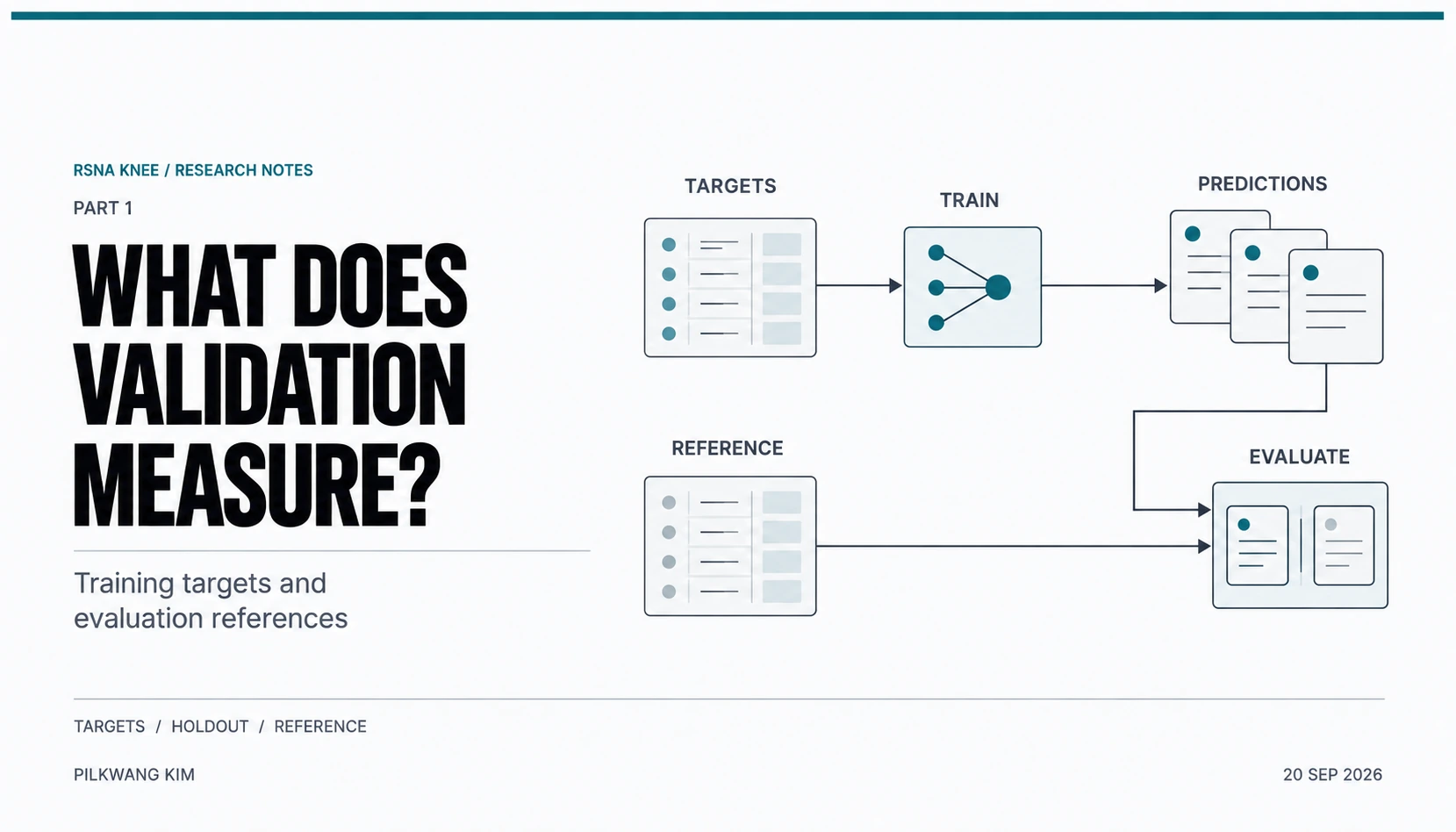
For a study, I distinguish the soft training target $q_i^{(\ell)}$, the image model’s prediction $p_i=f_\theta(X_i)$, and a binary validation reference $y_i^{(r)}$. The superscript $\ell$ identifies the training-label construction; $r$ identifies the reference interpretation. The training target may contain probabilities or uncertainty values, whereas the validation reference must define positive and negative cases for AUC. Changing either changes the comparison, even when the MRI inputs stay fixed.

The first label improvements were substantial. On the 58 supplied expert-annotated studies, rule-derived labels achieved about 0.812 macro AUC, compared with about 0.873 for a Sonnet report reader. Richer report interpretation was worth pursuing. The later rank-averaged Sonnet–Opus labels exposed the limit of using that agreement alone:

Comparison	Earlier setup	Revised setup
Label-table AUC on a 57-study expert panel	0.8700	0.8809
Image-model AUC on its annotated holdout	0.8400	0.8322

The label-table comparison uses a 57-study panel, rather than the 58 studies used for the earlier rule-versus-reader comparison.

The reader can use explicit wording, diagnostic conclusions, and descriptions of uncertainty. The image model must learn from the selected views and slices. A target table can agree more closely with a small reference panel while changing the prevalence, confidence, or distinctions presented throughout the training set. This experiment did not identify a single cause of the model’s decrease. It did show why a good label-table score cannot replace a downstream training comparison.

Rank transformations of predictions and training targets

AUC depends on ordering. Applying the same strictly increasing transformation to one predictor’s scores preserves its positive–negative ordering, apart from numerical ties. This property is why I consider rank averaging when combining outputs whose scales differ.

A percentile rank is nevertheless a position in a distribution, not a probability. An example at the 60th percentile need not have a 60% probability of containing a finding. If most reports are negative for that finding, even many negative examples can receive middle-ranking values. Replacing probability targets with ranks therefore changes what the image model is asked to predict.

Binary cross-entropy uses the target value directly:

\[\mathcal L(q,p)=-q\log p-(1-q)\log(1-p).\]

For a model logit $z$, with $p=\sigma(z)$, its gradient is

\[\frac{\partial\mathcal L}{\partial z}=p-q.\]

Consider an illustrative example. The model currently predicts 0.20. With a target of 0.02, the logit gradient is +0.18, so gradient descent lowers the logit and predicted probability. If a rank transformation changes the target to 0.60, the gradient becomes −0.40: the same image now pushes the prediction upward. A transformation that preserves the label table’s AUC can reverse its training signal.

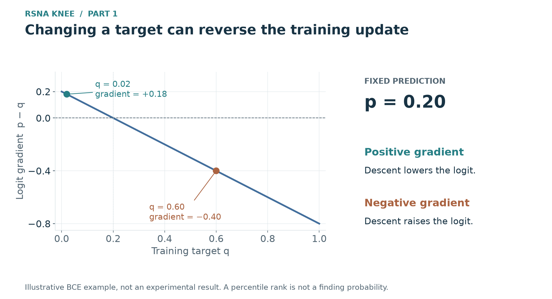Figure 1. Illustrative values at a fixed prediction of 0.20. The two target encodings produce opposite update directions. This explains the loss, rather than estimating the cause or size of an observed model-score change.

Rank-based targets can still be useful. They need to be evaluated as a changed learning task, rather than treated as probabilities with an unchanged meaning. Confidence weighting makes a different change: it leaves the target values alone and alters how strongly each cell contributes to the loss. The next label experiment makes that distinction concrete.

Report omissions and training loss

The finer, or wide, label schema was intended to express more of the report’s uncertainty. Its first difficulty concerned the order of two meanings: an explicit denial and a finding the report never raised. In the small annotated panel, 4.1% of 196 explicitly denied finding cells were positive in the image annotation, compared with 13.6% of 177 unmentioned cells. Those pooled cells were not independent patients, but the contrast gave a concrete reason not to assign silence a stronger negative meaning than an explicit denial.

The initial table had reversed that order. I first interpreted its low correlation with the earlier labels, 0.557, as evidence of a different supervision signal; correcting the ordering raised the correlation to 0.878. Only after that correction could I usefully compare whether a finer schema improved image supervision.

The corrected table’s model still lost roughly 0.013–0.027 under the report-derived references. Its target-level results were much less uniform:

Findings grouped by how often reports left them unmentioned	Mean model AUC change
Five findings with an omission rate below 11%	+0.0068
Six findings with an omission rate above 30%	−0.0323

The remaining finding lay between those omission groups. Across findings, the reported rank correlation between omission rate and score change was −0.657. Extra label detail appeared useful where reports usually spoke, while the losses concentrated where reports often said nothing.

The loss suggests a testable explanation. The example weight was $w_i=0.25+0.75c_i$, where $c_i$ was the reader’s confidence. Even a very uncertain cell retains positive weight. Its logit gradient is $w_i(p_i-q_i)$: the model is still pushed toward the assigned value, just less strongly. When many cells are unmentioned, reproducing their assigned values can account for a substantial part of training.

A matched run that masked low-confidence wide-label cells improved by a reported +0.0083, with a paired interval of [+0.0055, +0.0112].¹ Fracture, unmentioned in about 66% of its report cells, gained +0.0475; Contusion gained +0.0138. The result suggests that deciding which cells to learn from matters alongside deciding how finely to encode them.

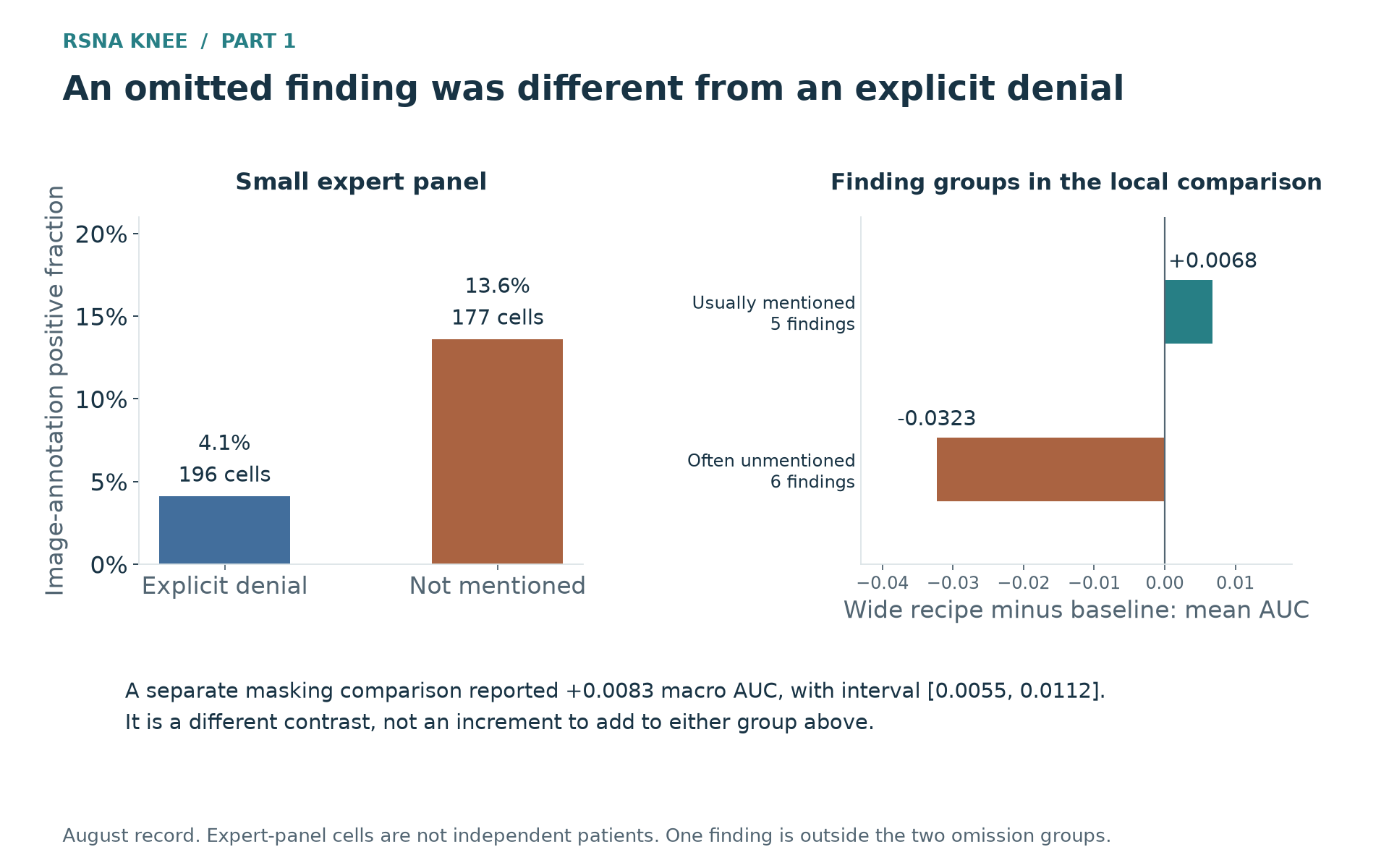Figure 2. The omission groups and the masking comparison describe different comparisons: the first compares the corrected wide-label model with its baseline, and the second changes masking within the wide-label recipe. The masking interval is the reported study-resampling interval for that matched comparison. It is not an uncertainty estimate for all label schemes.

Evaluation needs the same care. A reference that marks unmentioned findings negative can reward a model for reproducing that reporting habit. Removing those cells from training may reduce agreement with the reference without worsening image-finding prediction. Masking also removed studies with no supervised cells left—40 under the wide table—so comparisons must use shared eligible studies. Target-level changes and multiple references can help locate the disagreement; neither a label-table score nor a single masked-run score establishes clinical accuracy.

Crop, resolution, and anatomical coverage

Pixel-side experiments supplied a useful contrast. At a fixed 336-pixel image size, changing the physical crop from 130 mm to 100 mm gained about 0.005 in paired comparisons of held-out predictions. Going wider to 160 mm lost 0.0015; cropping further to 80 mm gained only 0.0019. The useful crop was in the middle of the tested range. Increasing apparent detail helped until removing context or anatomy became a competing cost.

Increasing input resolution produced a related effect. Increasing the grid from 336 to 448 pixels at a 130 mm crop gained about 0.003. Combining 448 pixels with the 100 mm crop gave about +0.0053, almost the same as the 100 mm crop at 336 pixels. Adding the two gains as if they were independent would exaggerate the combination’s value.

The representation explains why overlap was plausible. The nominal output pitch is the physical width divided by the grid width: 448 pixels over 130 mm gives about 0.290 mm per output pixel, close to 336 pixels over 100 mm at 0.298 mm. Both changes place a small structure across more input pixels. This is a property of the resized input, not a claim that interpolation improves the scanner’s acquired resolution.

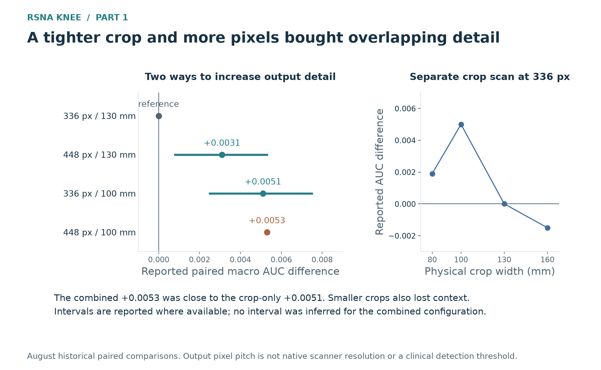Figure 3. Rounded effects from the paired comparisons, relative to 336 pixels and a 130 mm crop. The combined change gains little beyond the smaller crop alone. Similar output pitch explains a shared effect, while the different field of view means the two representations are not equivalent.

Pitch does not explain the entire difference: the 336-pixel, 100 mm representation beat the nearly pitch-matched 448-pixel, 130 mm representation by about 0.002. Cropping also changes which anatomy and background enter the model. I therefore favor the smaller representation. The larger grid has not shown enough additional value in this combination to justify its extra computation.

The image-input comparisons were also less sensitive to the reference labels than the reader swaps. In the tested set, pixel-side deltas varied across references by about 0.0002–0.0009, while label-side deltas varied by 0.0068–0.0073 and sometimes changed sign. This does not establish any reader as ground truth. It helps distinguish changes whose direction survives a different reference from those that need a more cautious interpretation.

OOF predictions and reference labels

Out-of-fold predictions reduce the optimism from evaluating images used in training. With five folds, each study is predicted by a model trained without its fold:

\[p_i^{\mathrm{OOF}}=f_{\theta_{-k(i)}}(X_i),\]

where $k(i)$ is the study’s fold. I also grouped repeated report text to reduce one route for duplicated information across folds. This supplies held-out image predictions across the cohort; it does not turn report-derived references into independent clinical truth.

For a specified predictor or ensemble $P$, a reference-label score is

\[S_r(P)=\frac{1}{12}\sum_{t=1}^{12} \operatorname{AUC}\!\left(y_t^{(r)},p_{P,t}^{\mathrm{OOF}}\right).\]

The reference determines which studies count as positive and negative for each target. Changing how a reader interprets an uncertain phrase or an omission changes the positive–negative pairs used by AUC. The image predictions can stay identical while the measured score changes.

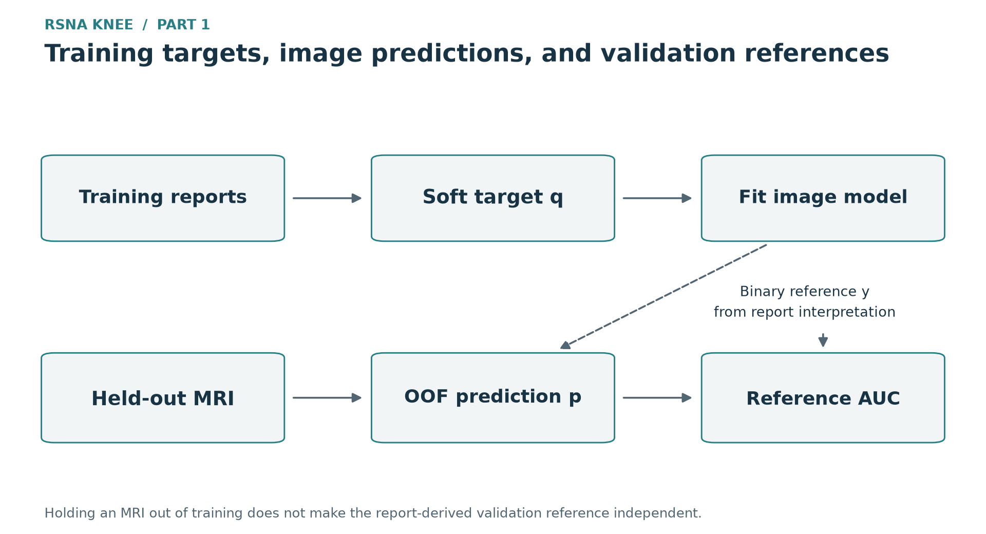Figure 4. Image holdout and reference independence are separate properties. OOF addresses whether the image learner fitted a study; it does not establish how accurately or independently a report reader defines that study’s findings.

The distinction matters most when the training target and reference share a reader or a related interpretation. A higher score establishes better agreement with that interpretation. The small expert panel supports direct examination of annotated cases; report-derived references support cohort-wide candidate comparisons; Public AUC evaluates a submitted system on the competition’s scored cases. Together they can reveal where judgments disagree. One measurement cannot replace another.

Limits of the minimum-AUC objective

I initially tried to avoid improving under only one reference by maximizing the minimum score:

\[S_{\min}(P)=\min_r S_r(P).\]

The rule looks conservative: improve the lowest score before receiving credit. But the three scores use different reference labels. Their absolute levels can differ for reasons unrelated to a candidate’s performance. If one reference stays lower by much more than candidates move, it determines the minimum throughout the comparison.

That was the observed behavior. Among 200 sampled candidate ensembles, the rule-based v1 score was the minimum in all 200. Within that tested set,

\[S_{\min}(P)=S_{\mathrm{v1}}(P).\]

One recorded candidate shows the consequence:

Reference	Starting ensemble	Change	Candidate ensemble
Rules, v1	0.8210	+0.0058	0.8268
Opus reader	0.8791	−0.0048	0.8743
GPT reader	0.8835	−0.0046	0.8788

Values and changes are rounded independently; adding displayed entries can differ in the final digit.

The candidate improved the minimum while worsening both other scores. Their declines were too small to close their large level gap with v1, so neither decline affected the objective. A rule intended to balance references instead rewarded one interpretation exclusively in this region.

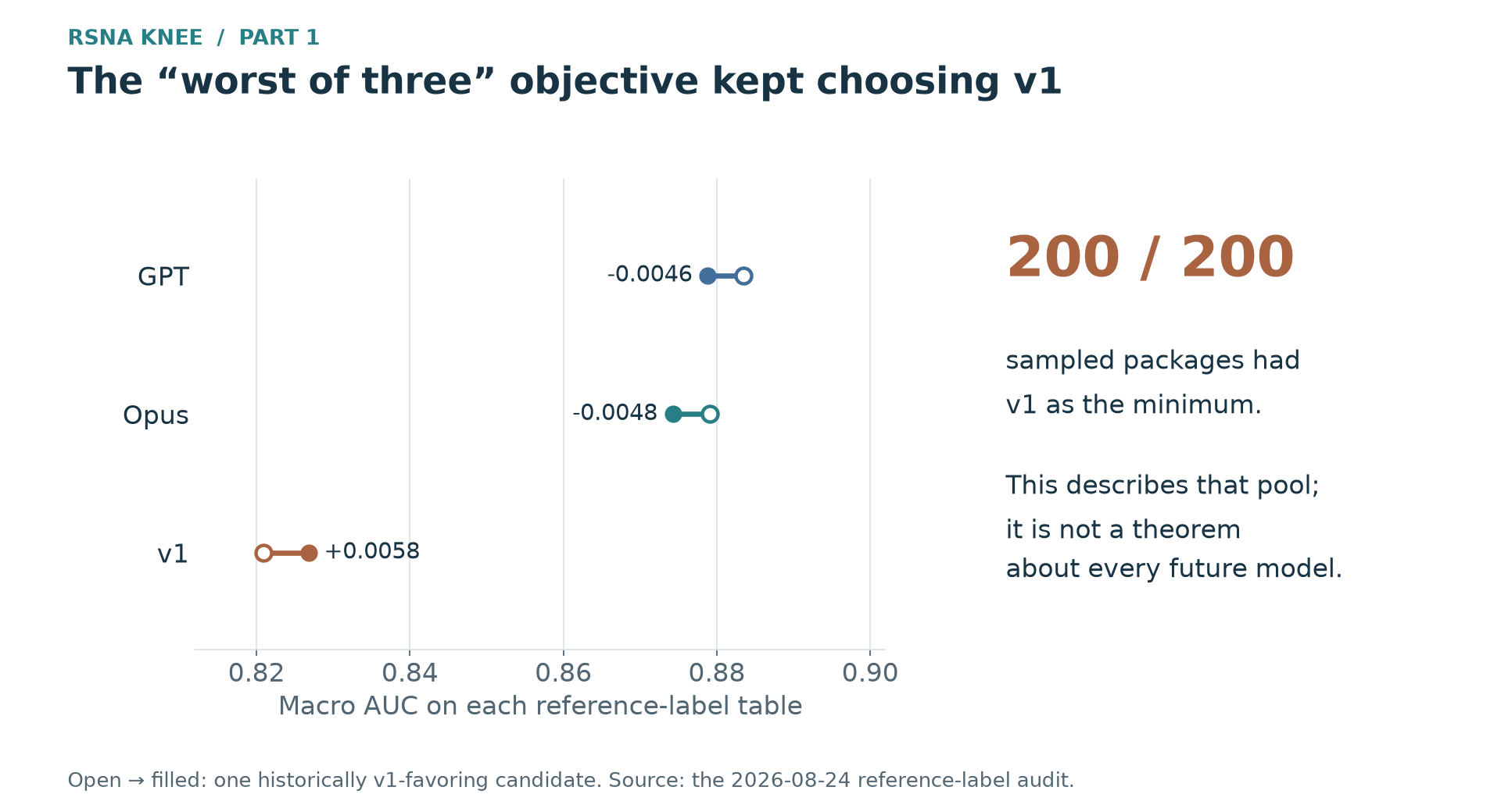Figure 5. The recorded example and the 200-candidate check expose the same mechanism: v1 controls the minimum because its score level is lower. This conclusion is limited to the evaluated candidates.

In response, I replaced the minimum with the mean of Opus and GPT as my working primary score, retaining v1 as a separate veto check. Gains and losses under Opus and GPT can now affect selection. This does not make the two references independent or uniquely correct. I still need to interpret them alongside individual findings, annotated cases, and competition results.

Encoder adaptation and further training

A declared reference does not settle whether a new model has received enough training. With rad-dino, I had to choose between further adaptation and spending that time on another candidate. The encoder had been pretrained on chest X-rays and could replace DINOv2-base without changing the input architecture. I expected that holding the rest of the recipe fixed would isolate the effect of initialization.

Under thirty epochs with six unfrozen blocks and a backbone learning rate of $8\times10^{-6}$, rad-dino was weak. Its five-fold OOF was not selected in any of the five folds under any of three references. Yet its recorded best epochs were 29, 29, 30, 30, and 29. The comparison had fixed the adaptation budget at a recipe developed for DINOv2. A different initialization might need a different amount or form of fine-tuning.

Two first-fold retests addressed that concern:

rad-dino recipe	Best first-fold AUC against the GPT-derived reference
Original 30 epochs	0.8356
Continue the same run to 60 epochs	0.8417
Open all 12 blocks, learning rate $2\times10^{-5}$, 30 epochs	0.8429
DINOv2 control	0.8795

The extended run peaked at epoch 48 and ended at 0.8393. The two retests recovered about 0.006–0.007, but left a substantial gap to the control. Having measured how much additional training recovered, I am giving this line a lower priority. I am keeping its completed OOF for combinations with other models.

A best epoch near the end does not establish insufficient training by itself. A cyclic learning rate becomes small at the end of each cycle, so peaks can accumulate there even without a large gain from another cycle. Here I actually extended training and observed performance fall after its new peak. Opening all blocks and changing the rate tested another adaptation strategy; the two retests do not establish that every possible recipe would fail.

I also examined the ensemble result rather than deciding from standalone performance alone. In the local comparison, adding rad-dino to the existing seven-family package reduced the worst-reference score by only 0.0007, far less than its standalone deficit. A small loss does not establish useful complementarity: a low mixing weight also limits a weak member’s effect. Whether more adaptation would help was a separate question worth a bounded retest. With its recovery now measured, I intend to spend the next substantial training effort on another candidate.

Criteria for the next comparisons

In the next experiments, I want to ask what changed as well as whether AUC rose. For supervision, that means separating the reader’s ordering from target values and loss weights. For image inputs, it means checking whether two changes supply similar detail or different anatomical coverage. For an encoder, I need to distinguish performance under the incumbent recipe from performance after adequate adaptation.

I am not choosing a final model yet. I plan to train models that use different features and obtain complete OOF predictions for each. Those predictions will support comparisons of useful combinations and which ones are worth evaluating under the nine-hour inference limit.

1. The record for this comparison does not identify the scoring reference. Its reported local gain is therefore not directly comparable with gains on my current primary score or with clinical/Public performance. ↩︎