RSNA Knee, Part 2: Ensembles Under a Nine-Hour Limit

Select a figure to enlarge it. On small screens, wide tables and equations scroll horizontally.

An ensemble is a calculation applied to a set of predictions. Its quality depends on which predictions enter, how their numerical scales are combined, and which ranking errors the combination changes. The number of checkpoints is only an indirect description of that calculation. The same models can produce different study rankings under different reducers, and a larger collection can perform worse than a well-chosen subset.

The strongest compact candidate I can select now combines two locally trained model families. It has scored Public 0.940 with rank averaging and 0.941 with probability averaging, at a planned inference cost of 207.7 minutes. Broader candidates have used much more computation without exceeding it on Public. These results raise two related questions: how to train models that add useful information, and how to choose among their combinations when the local estimate and the computational cost favor different candidates. A representation experiment and the first ensemble comparison show why I cannot answer either question from a standalone score.

Prediction matrices and aggregation

For one finding $t$, write the available predictions as a matrix $P^{(t)}$: studies occupy rows, and prediction sources occupy columns. Each column must refer to the same study keys and an understood evaluation procedure. In local comparisons, a complete family supplies OOF predictions from five fold models, with each study predicted by the model that excluded its fold. This makes the rows comparable without using that study’s own fitted prediction.

A weighted probability mean and a weighted rank mean are different functions of this matrix:

\[\begin{aligned} s^{\mathrm{prob}}_{it}&=\sum_j w_{jt}P^{(t)}_{ij},\\ s^{\mathrm{rank}}_{it}&=\sum_j w_{jt}R_{jt}\!\left(P^{(t)}_{ij}\right),\\ w_{jt}&\geq 0,\quad \sum_jw_{jt}=1. \end{aligned}\]

Here $R_{jt}$ converts a source’s predictions for one finding into percentile ranks across the evaluated studies. Probability averaging retains differences in score spacing. Rank averaging replaces those distances with relative positions before combining the sources. A monotonic transformation preserves an individual predictor’s AUC when its ordering and ties are preserved, but applying transformations separately before addition can change the sum’s ordering.

This distinction also explains why standalone AUC does not determine ensemble value. For a positive–negative pair, let $d_j=P_j(x^+)-P_j(x^-)$. A probability mean ranks the pair according to $\sum_jw_jd_j$. A second model helps when it reverses sufficiently many incorrect pair orderings without overturning too many correct ones. A model with slightly lower standalone AUC can therefore improve a stronger model; a highly ranked model can be redundant if both make the same consequential mistakes.

Prediction correlation summarizes similarity, not whether disagreements are correct. A low correlation can reflect complementary information or simply a poor predictor. Because the metric averages twelve finding-level AUCs, the useful disagreements can also differ by finding. To measure a contribution, I need predictions on the same studies combined with the operator I intend to use. Another encoder or seed has no fixed ensemble value by itself.

I use a flat roster for the same set of families across all twelve findings, and target-specific selection for separate sets by finding. These are different choices of membership, regardless of whether their predictions are combined by probability or rank averaging.

Averaging levels, fold models, and executed membership

If two families each contain five models, an equal probability mean of their family means equals a flat ten-model mean. That equality depends on equal family sizes and no intervening transformation. Unequal family sizes require different outer weights to reproduce a flat mean. Reranking a family mean or inserting another nonlinear transform generally produces a different calculation; changing weights alone does not restore the equality.

OOF and hidden inference also use different eligible predictions. A training study has one held-out model per family; averaging all five fold models on that study would introduce in-sample predictions. At hidden inference, all five models may contribute. The local construction must retain its held-out condition, while the deployment definition specifies the actual fold-model reducer.

One rehearsal exposed a more basic mismatch. On September 22, a 1,322-study run loaded 45 members, but an older per-finding list let only 10–25 contribute to each output. Both new configurations were absent from every output. On 4,339 shared OOF studies, the intended flat nine-configuration composition scored 0.8817 on the primary metric, against 0.8785 for the older composition. Correcting membership made the declared comparison possible; that local difference did not estimate a hidden-score gain.

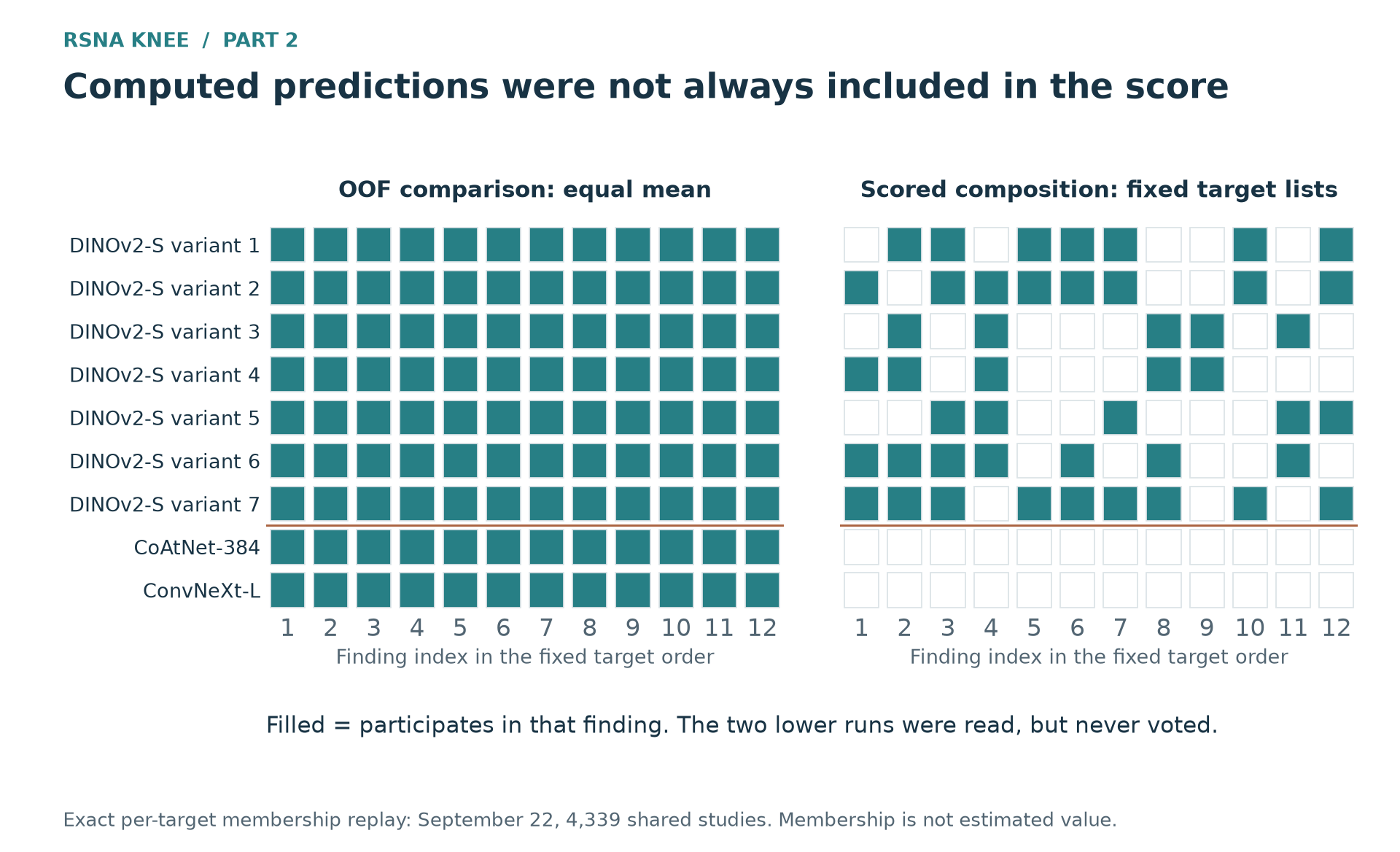Figure 1. The intended composition includes all nine configurations in all twelve findings. The recorded mask uses seven configurations, with 10–25 participating members out of 45. Loading a model did not ensure that it affected the prediction.

The same rehearsal shortened 26 members from ten windows to nine under an internal eight-hour timer. I removed that adaptation. The execution order or chunk sizes may change, but the selected models and windows must remain fixed. Otherwise, the local estimate and the scored run describe different predictors.

Complementary model families

Combination analysis needs the candidate predictions before it can test their complementarity. A promising first fold is not enough for comparison across the bank; a complete family supplies held-out predictions on the same studies as the existing models. The earlier decision is harder: which learning system is worth training to produce those predictions?

A public Raptor recipe suggested one such system. It combined a CoAtNet encoder, a 64-slice representation, attention over windows, and a training setup adapted to that representation. I retrained it on my folds to obtain usable OOF, rather than treating a competition-trained public checkpoint as though it had excluded my validation studies.

The early component tests were unfavorable. With my existing classification head, CoAtNet scored 0.8663 on the first fold against GPT report-derived reference labels, below the DINOv2-small control’s 0.8795. Keeping that head while adopting the public 64-slice input produced 0.8322. Those experiments tested specific transplanted combinations. They did not establish how the complete recipe would behave.

The interaction was understandable. An encoder maps image windows to features; the head must aggregate those features into finding probabilities. Changing the windows changes both the distribution and the arrangement of the head’s inputs. A head designed around a few selected views may use a longer sequence poorly. A learned window-attention head can instead weight observations from that longer sequence, provided the features and fine-tuning allow it to identify useful evidence.

I therefore trained the 64-slice representation with the public lineage’s attention head and fuller fine-tuning. At epoch 16, the first-fold score reached 0.8701, an increase of 0.0379 over the input transplant. The comparison supported continuing the coupled recipe, although the changed fine-tuning prevented attribution to the head alone.

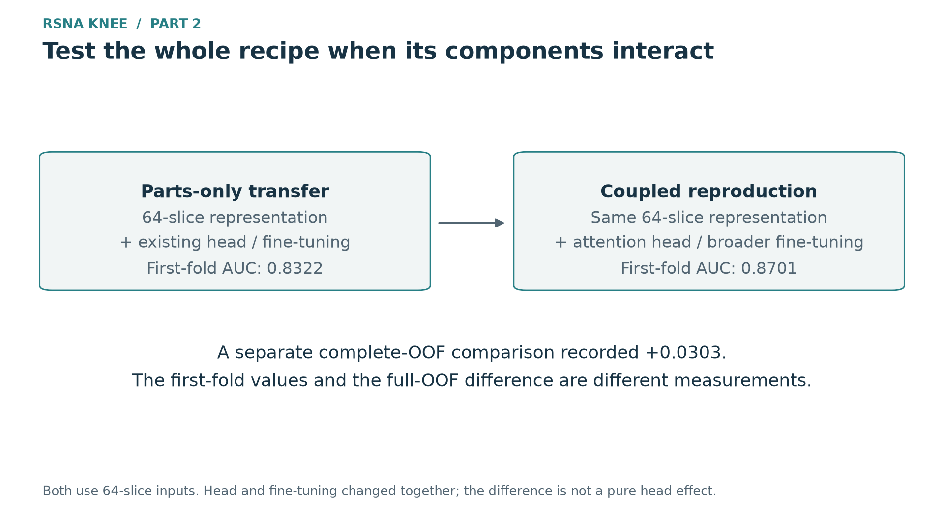Figure 2. The first-fold scores 0.8322 and 0.8701 use the same report-derived reference labels. Both use the 64-slice representation; the latter is an intermediate checkpoint after changing the head and broadening fine-tuning together. The completed OOF comparison is a separate result.

The five folds finished on September 23. On the primary metric—the mean AUC against GPT and Opus reference labels—the coupled family exceeded the same-input, original-head family by 0.0303. It remained 0.0091 below the baseline family alone. Yet its correlation with the deployed composition was 0.789, and combination selection included it in all five outer folds. That was evidence of useful complementarity in the evaluated procedure, despite the weaker standalone result.

The resulting held-out predictions let me compare the coupled recipe with the other families. A different architecture name, a successful implementation, or a higher first-fold score would not be enough for that comparison. The result is a reason to test interacting parts together, rather than reject the whole recipe after inserting one component into an otherwise unchanged system.

Dense inputs and optimization interactions

Another set of experiments showed why the training recipe could not be separated from the representation by inspection alone. Two models with a denser 336-pixel, 30-slice input had large first-fold losses: about −0.054 for ConvNeXt-large and −0.125 for DINOv2-large. The proposed change sounded like “more slices.” The actual recipes also changed crop, fine-tuning depth, learning rate, schedule, and precision. They tested whole systems, so the losses did not identify which change was responsible.

A small DINOv2 experiment isolated the suspected interaction. I changed the backbone learning rate from $8\times10^{-6}$ to $2\times10^{-5}$, opened the full encoder depth, and tested their combination while keeping the other baseline settings fixed. On 881 held-out studies, one consistent comparison against the stored baseline gave:

Learning rate	Fine-tuning depth	Primary AUC
Original	Partial	0.8760
Raised	Partial	0.8374
Original	Full	0.8714
Raised	Full	0.7288

The primary score was the mean of the Opus- and GPT-reference AUCs. Raising the rate alone hurt substantially; opening the depth alone had a much smaller effect. Their combination was much worse than adding those two losses. Writing the four scores as $s_0,s_R,s_D,s_{RD}$, the interaction was

\[I_{R\times D}=s_{RD}-s_R-s_D+s_0=-0.1040.\]

A paired four-arm bootstrap gave an interval of [−0.1154, −0.0926]. These resamples describe variation among the held-out studies, not variation across independently trained seeds. Within the tested recipe, however, the magnitude was enough to change the next experiment: restore the learning rate before treating the dense representation as the source of the whole loss.

That repair still needed a direct test. The two-factor experiment used the original input, whereas the failing dense configuration also carried the new geometry, schedule, and precision. I kept those settings and full-depth fine-tuning, changing only the backbone rate back to its original value. If the suspected interaction explained much of the failure, the repaired configuration should recover far more than the rate’s standalone effect.

It did. Relative to the same stored baseline, the complete dense configuration went from −0.1283 to −0.0283, a recovery of +0.1000 [0.0897, 0.1111]. The remaining result was close to the geometry-only arm, −0.0293; their difference was +0.0010 [−0.0041, +0.0063].

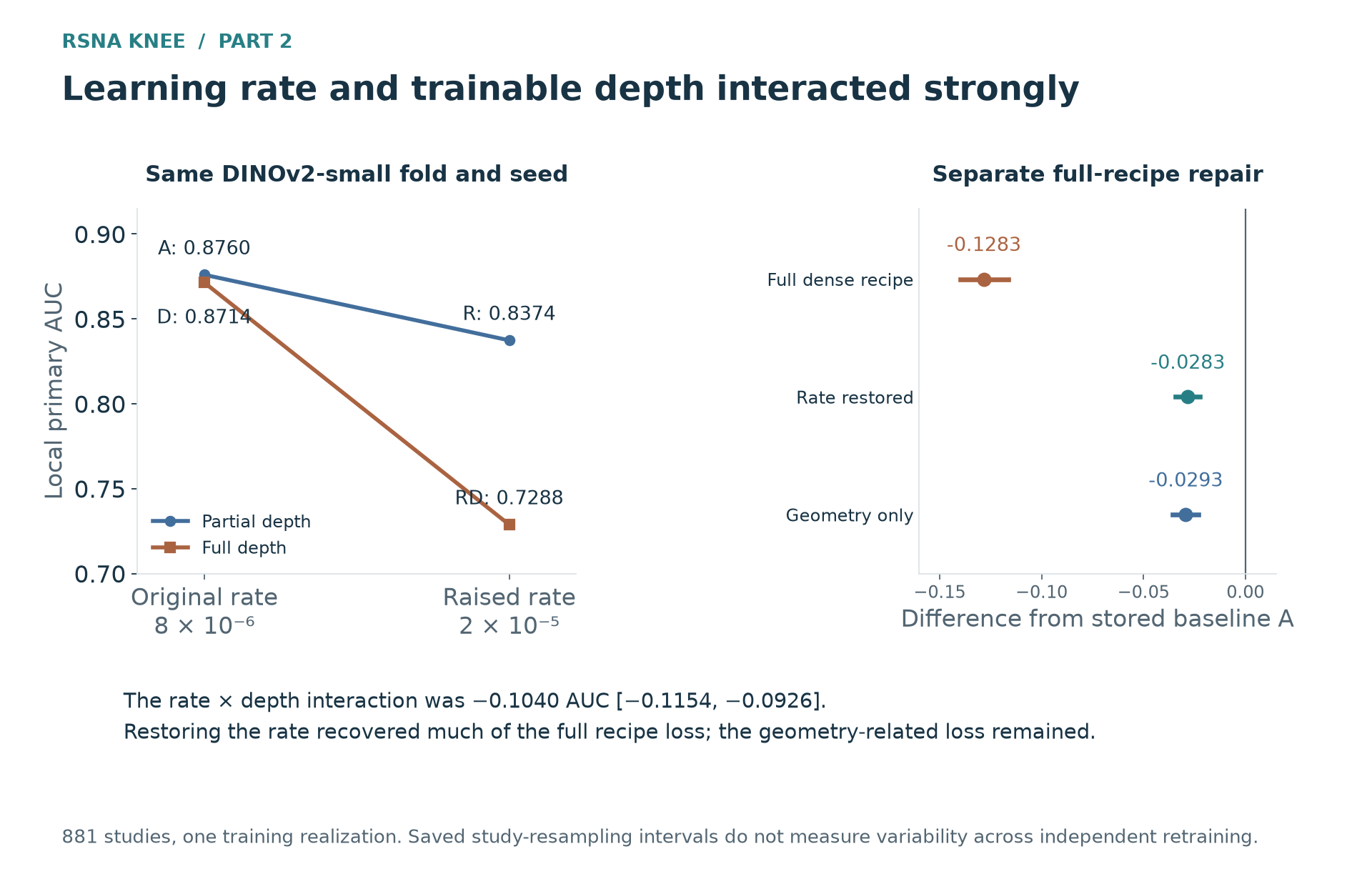Figure 3. Left: four matched conditions show a large negative rate-by-depth interaction. Right: restoring the rate in the full dense recipe recovers much of its loss, while a residual geometry cost remains. All values use the same stored-baseline comparison; the results concern one DINOv2-small fold and seed.

The repaired dense recipe is worth testing further, but this is not a blanket endorsement of more slices. The geometry bundle still loses about 0.03 under these references, and the experiment does not separate slice count from crop and band coverage. Nor does it establish the same numerical interaction in a larger encoder. For the next large-model comparison, I need that encoder’s own established optimization settings. The original test changed the representation together with a poor optimization combination; it cannot decide the representation question on its own.

Inference routes and cost constraints

The mathematical selection problem has both a statistical objective and a resource constraint. Let $c$ specify the models, reducer, and weights, and let $S_D(c)$ be macro AUC against the declared reference labels on studies $D$. The intended feasible problem is

\[\begin{aligned} &\underset{c\in\mathcal C}{\operatorname{maximize}}\ S_D(c)\\ &\text{subject to}\quad T_{\mathrm{route}}(c)\leq 540\ \text{minutes}. \end{aligned}\]

The reference labels make this a particular local objective, not direct access to the hidden clinical targets. The time constraint concerns the complete computation on two T4 GPUs. Both definitions matter: changing the reference can change the preferred composition, while changing the inference route can change whether that composition fits.

Runtime is not an independent price attached to every family. Models with compatible inputs can share decoded images. Adding another model to an existing input group may therefore cost less than introducing a new crop or slice schedule. Conversely, a small network can require substantial additional preparation if its representation cannot be reused.

For a staged execution with non-overlapping accounting terms, a useful decomposition is

\[\begin{aligned} T_{\mathrm{route}}(c)={}&T_{\mathrm{setup}}+T_{\mathrm{decode}}(c)\\ &+T_{\mathrm{two\ GPUs}}(c)+T_{\mathrm{aggregation}}(c). \end{aligned}\]

The two-GPU term depends on scheduling. If different members run on separate devices, the slower lane determines when the stage finishes. Unequal workloads, serial decoding, and aggregation prevent a doubling of model throughput from halving the total time. Keeping decoded groups in memory can avoid repeated work, but their simultaneous residency can increase peak memory. Model selection, shared preparation, scheduling, and memory therefore have to be priced together.

Before a full run, I have an estimate $\widehat T_{\mathrm{route}}$, rather than the exact hidden runtime. The selection program uses that estimate to propose compositions, but a 540-minute planning estimate does not certify completion. Deliberate trials above the planning limit test whether a useful exact composition can finish; they do not extend Kaggle’s actual nine-hour allowance.

The observations illustrate the distinction. A candidate planned at 599.8 minutes failed with a certified time limit. Another planned at 567.8 minutes completed and scored 0.937. Their send-to-result intervals were about 9.18 and 8.89 hours, including platform and collection delay. Different contents and execution routes prevent treating those two points as a universal runtime boundary.

Cross-fitted selection and fitted rosters

The September 20 bank already supplied a reason to compare replacements, not just additions. On 4,339 shared studies, a descriptive search over 76 complete configurations produced these fixed candidates:

Candidate	Configurations	Decode groups	Primary AUC change versus R1
Current R1	9	3	—
Selected top eight	8	2	+0.0017
Selected top nine	9	3	+0.0020
R1 plus the window-bag family	10	4	+0.0010
Equal combination of all available configurations	76	13	−0.0092

The smaller selected set improved the measured score while requiring fewer decoding groups. Adding the bag family was another useful candidate, but it was not the best alternative simply because it preserved every incumbent. Conversely, the poor result from averaging everything said little about what a well-chosen subset could achieve. The value of a complete OOF bank was the ability to construct those different predictions on the same studies.

These were fitted comparisons: the same predictions had helped choose the shortlist. With a complete OOF matrix, thousands of combinations can be compared without retraining the image models, but that convenience creates a statistical problem. If I choose the maximum of $S_D(c)$ over many candidates and report its score on the same rows, favorable accidents enter the choice. More flexible weights or finding-specific membership give the selection more ways to fit those accidents.

I used cross-fitting for the combination procedure. For outer fold $k$, selection used the other four folds’ OOF predictions and evaluation used the omitted fold:

\[c^{(-k)}=\operatorname{Select}(\mathrm{OOF}_{-k}), \qquad \widehat p_i^{\,\mathrm{cf}}=g_{c^{(-k(i))}}(P_i).\]

The selected composition could differ between outer folds. I pooled their held-out predictions to calculate macro AUC, evaluating how the procedure chose under that pool, objective, and runtime accounting. I could then fit a final roster using all available OOF. Its fitted score answered how well that particular choice matched the data used to choose it; it was a different result from the cross-fitted procedure estimate.

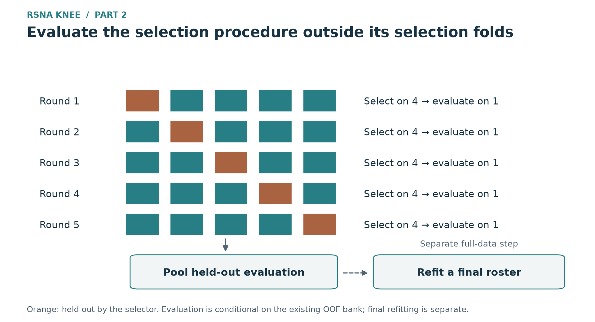Figure 4. Four folds select and one fold evaluates, repeated five times. A separate all-OOF fit assembles the final roster. The procedure operates on an existing prediction matrix; it does not retrain every base model inside the outer folds.

What is held out, and what a fixed-roster interval measures

The existing base models had ordinary five-fold training. Models predicting other folds could have learned from the outer fold’s studies, even though the selector did not directly use its evaluation labels. Cross-fitting the combination therefore evaluates selection conditional on the existing predictions and prior development. It is not a fully nested assessment of the whole learning process.

Pooled macro AUC is also different from the mean of five fold AUCs: pooling includes positive–negative comparisons across folds, where score-range differences may matter. The procedure estimate must specify which calculation it uses.

A paired bootstrap with the chosen roster fixed resamples studies for those predictions. It does not rerun selection or account for every possible roster change. The interval is conditional on the chosen roster and reference. It does not measure variation from repeatedly choosing a new roster, or estimate Public noise.

Local estimates and the first scored comparison

By September 23, the candidate pool contained 83 configurations. I compared flat and target-specific selection while restricting both to input groups already exercised in a scored run. Under the 540-minute planning cap, target-specific selection had the higher cross-fitted primary gain: +0.0090 against flat selection’s +0.0067. The difficult choice was whether that larger estimate justified taking the much larger construction first.

Changing the planning cap made the difference more informative:

Planning cap	Flat-selection gain	Target-specific gain
240 minutes	+0.0068	+0.0086
300 minutes	+0.0067	+0.0057
360 minutes	+0.0067	+0.0074
420 minutes	+0.0067	+0.0090
480 minutes	+0.0067	+0.0083
540 minutes	+0.0067	+0.0090

These are held-out procedure results on the same declared reference objective, not Public-score predictions. Flat selection changed little. The target-specific procedure chose different combinations as the cap moved, and at 300 minutes its results included fallbacks in two outer folds. A larger cap expands the possible training choices; it does not require the chosen predictor’s held-out AUC to increase monotonically. The curve exposed sensitivity to the selection conditions, rather than supplying a new estimate of Public noise or an automatic reason to reject target-specific selection.

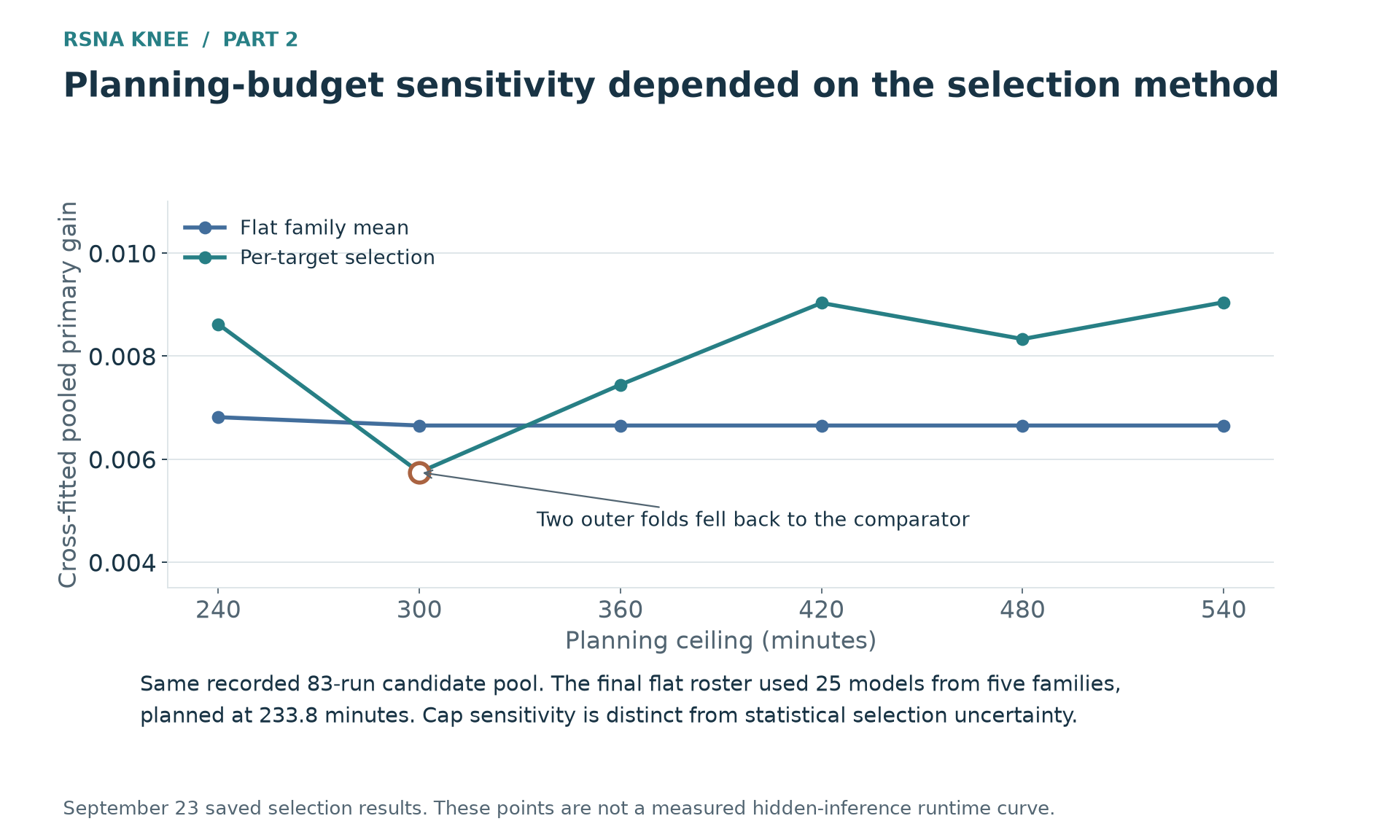Figure 5. The September 23 pool gives nearly stable flat-selection gains and a more cap-sensitive target-specific procedure. The 300-minute point includes two fold fallbacks. The earlier 76-configuration table and these 83-configuration curves are different pool snapshots.

The first trial used the flat construction: five families, 25 fold models, two input groups, and 233.8 planned minutes. Its members combined a small DINOv2 reader-label baseline, its fuller-depth variant, a hybrid-label variant, ConvNeXt-large, and the coupled 64-slice Raptor family. This was a new subset of the bank, not the previous package with one more family attached. It used less than half the planning cap while keeping the more ambitious target-specific option available for a later comparison.

The submitted system reached Public 0.928 on September 23, up from 0.921; an external RadImageNet component was still included. A later target-specific composition scored 0.931. Those outcomes justified further selection comparisons, but they do not provide a general conversion from local gains to Public gains. Contents and execution changed together. I therefore also tested a compact pair, rather than assume that the larger selected rosters made the best use of the bank.

The compact two-family ensemble

The strongest small combination paired an 80-slice gated model trained on GPT-derived labels with a 64-slice coupled model trained on publicly released Raptor labels. Both had complete OOF on my folds. Their standalone Public scores were 0.935 and 0.932. The ten fold models, combined by a flat rank mean, scored 0.940 on September 30. Probability averaging the same ten members scored 0.941 on October 3. Neither composition included an external checkpoint component.

At 207.7 planned minutes, the pair was substantially cheaper than the broad alternatives. A 539.8-minute composition scored 0.935; the completed 567.8-minute composition scored 0.937. Other broad tests also remained below the pair, even when report-derived reference labels preferred them locally.

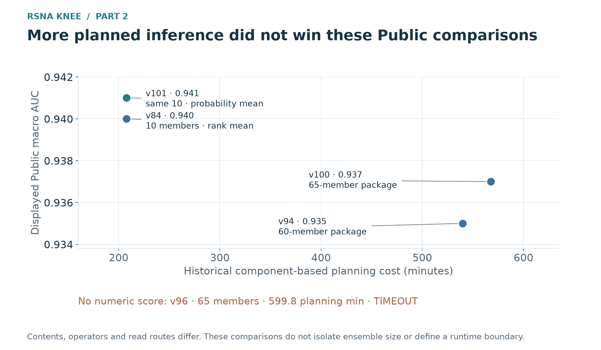Figure 6. The pair’s rank and probability means scored 0.940 and 0.941 at the same 207.7-minute planning cost. Broader candidates planned at 539.8 and 567.8 minutes scored 0.935 and 0.937. The 599.8-minute trial timed out and supplied no AUC. Contents and operators differ across these comparisons.

The compact pair is now a useful candidate, but its result does not establish a general preference for fewer models. The broad compositions change which predictions dominate and how their errors combine. I am keeping all complete OOF: a new family or evidence for a different objective may favor another subset. If I compared only additions to the current favorite, I would miss replacements such as this pair.

The operator comparison supports probability averaging for these fixed ten models: its displayed score increased from 0.940 to 0.941. It does not establish a best general weighting rule. I want a few declared Public comparisons to check whether a proposed improvement holds on the competition sample, without adjusting the weights after every small score change.

The cap comparisons helped me choose the first trial, and the dense-input repair separated an optimization failure from the representation question. The local objective is still unresolved. The Raptor-labeled family scored 0.932 against 0.920 for its GPT-labeled visual control, although the primary reference preferred the control. That disagreement also appears among the broader ensembles. I have a selectable two-family candidate and complete OOF from the other models, but I do not yet know why the local and Public rankings differ. My next comparisons need to examine the training targets and the reference labels, alongside the image models themselves.