BioHub Cell Tracking 작업 기록 1: Lineage Graph 학습과 평가지표에 맞춘 후처리

시리즈 안내와 참고 링크

• 대회: BioHub - Cell Tracking During Development
• 공식 평가지표: RoyerLab kaggle-cell-tracking-competition metrics.md
• 배경 기사: Biohub Calls on AI Community to Transform 3D Cell Tracking
• 영문판: BioHub Cell Tracking Working Note 1: Learned Lineage Graphs and Metric-Aware Repair
• 후속 글: BioHub Cell Tracking 작업 기록 2: Public 점수가 멈췄을 때 — OOF 기반 오류 분석

관련 공개 노트북

• Biohub Cell Tracking: Data Model, EDA, Baseline
• Biohub Cell Tracking: Learned Graph w Gap Recovery
• Biohub Cell Tracking: Blend Preprocessings

시리즈 소개. BioHub는 3D 현미경 영상에서 세포의 lineage graph를 복원하는 대회다. 라벨이 있는 학습 자료는 두 배아에서 촬영한 영상 199편이며, hidden test의 29%는 Public, 나머지 71%는 Private 점수에 반영된다. hidden test는 학습에 쓰이지 않은 배아에서 나온다. 각 편은 해당 기간의 기록을 따라가며, 나중에 확인한 사실과 회고는 따로 표시했다.

나중에 확인한 내용 — 2026-09-23. 이 글을 쓴 뒤인 7월 18일에 division metric의 매칭 조건이 강화됐다. Public 차이 ±0.002 이내를 동점으로 읽는 기준도 9월 5–6일에 정한 것으로, 7월 제출을 고를 때부터 쓰던 규칙은 아니다.

초기에는 고전적인 중심점 검출과 최근접 연결에서 출발해, 학습한 lineage graph에 보수적인 복원 규칙을 더하는 방식으로 발전했다. 7월 11일 무렵에는 개선을 판단하는 단위가 분명해졌다. 검출기나 간선 점수가 좋아지는 것만으로는 부족했다. 그래프 생성과 후처리를 거친 최종 출력에서 올바른 추적이 늘어야 했다.

그래프 \(G=(V,E)\)에서 노드는 한 시점에 검출한 세포이고, 간선은 시간에 따른 연결이다. 분열은 하나의 부모에서 두 딸세포로 갈라지는 모양으로 나타난다. 주석이 희소하기 때문에 영상에 분명히 보이는 세포에도 정답 표시가 없을 수 있고, 중간 시점의 검출 하나가 빠지면 lineage 전체가 끊어질 수 있다. 이런 조건이 학습과 복원 규칙을 함께 제약한다.

이 글은 7월 11일까지의 파이프라인과 초기 Public 관찰을 정리한다. 마지막 out-of-fold(OOF) 절에서는 각 영상을 그 영상 없이 학습한 모델로 예측하는 다음 단계의 설계를 다루며, 해당 평가는 아직 끝나지 않았다.

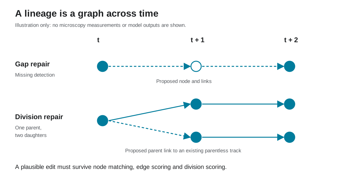그림 1. 설명용 모식도다. gap repair는 빠진 노드와 연결을 넣는다. 아래 division repair는 이미 검출됐지만 부모가 없는 딸세포 track에 부모 연결을 더하며, 새 딸세포를 검출하는 과정은 아니다.

---

1. 대회와 문제 설정

이 대회에서는 제브라피시 배아의 3차원 형광 현미경 영상에서 세포를 추적한다. 각 샘플은 짧은 3차원 시계열 영상이다. 알고리즘은 시점마다 세포를 검출하고, 같은 세포를 시간축으로 연결하며, 분열 사건을 lineage graph로 복원해야 한다.

발생 과정을 이해하려면 세포의 위치뿐 아니라 이동과 분열, 세대를 잇는 lineage를 함께 추적해야 한다. 하지만 실제 3차원 현미경 영상은 세포가 조밀하고 잡음이 많으며, 축마다 해상도가 다르다. 세포의 외형도 서로 비슷하다. 세포는 움직이며 모양이 바뀌고, 흐려지거나 다른 세포와 가까워졌다가 둘로 갈라진다. 사람이 전 과정을 추적하기에는 금세 한계가 온다.

입력 영상의 배열 구조와 물리적 축척은 다음과 같다.

sample.zarr/
  0/
    zarr.json
    c/{t}/0/0/0

shape: usually (T, Z, Y, X)
dtype: uint16
voxel scale:
  z = 1.62500 microns / voxel
  y = 0.40625 microns / voxel
  x = 0.40625 microns / voxel

학습 샘플에는 GEFF 형식의 희소한 lineage 주석이 제공된다.

sample.geff/
  nodes/ids
  nodes/props/t/values
  nodes/props/z/values
  nodes/props/y/values
  nodes/props/x/values
  edges/ids

핵심은 희소하다는 점이다. 영상에 보이는 모든 세포가 모든 프레임에 표시되어 있지는 않다. 따라서 일반적인 밀집 분할 검증만으로는 모델의 장단점을 제대로 판단하기 어렵다. 영상에서는 타당해 보이는 예측 세포도 희소한 정답 노드와 짝을 이루지 못할 수 있다. 결국 평가는 그래프 단위로 해야 하며, 후처리도 거짓 양성을 억제하는 쪽으로 설계해야 한다.

최종 제출물은 노드와 간선, 두 종류의 행으로 이루어진 CSV 파일이다.

id,dataset,row_type,node_id,t,z,y,x,source_id,target_id
0,44b6_xxxx,node,1,0,32,128,128,-1,-1
1,44b6_xxxx,node,2,1,33,130,125,-1,-1
2,44b6_xxxx,edge,-1,-1,-1,-1,-1,1,2

노드 행은 세포 검출 결과를, 간선 행은 시간축 연결을 나타낸다. 평가기는 이 CSV를 하나의 그래프로 해석한다.

---

2. 평가지표가 그래프 설계에 미치는 영향

평가기는 먼저 각 시점에서 예측 노드와 정답 노드를 중심점 사이의 물리적 거리로 짝짓는다. 복셀의 축척이 방향마다 다르므로, 거리는 반드시 마이크로미터 단위로 계산해야 한다.

\[d_{\mu m}(i,j) = \sqrt{ (1.625\Delta z)^2 + (0.40625\Delta y)^2 + (0.40625\Delta x)^2 }.\]

두 노드의 거리가 다음 한계 안에 있을 때만 짝을 이룰 수 있다.

\[d_{\mu m}(i,j) \le 7.0.\]

여기서 중요한 점은 반경 안의 모든 쌍을 정답으로 세지 않는다는 것이다. 평가기는 프레임 \(t\)마다 허용 거리 안의 후보로 최적 이분 매칭을 만들며, 한 노드는 반대편의 노드 하나와만 짝을 이룰 수 있다.

\[m_{ij}\in\{0,1\}, \qquad \sum_jm_{ij}\le1, \qquad \sum_im_{ij}\le1, \qquad m_{ij}=0\ \text{if}\ d_{\mu m}(i,j)>7.\]

예측 간선의 양 끝 노드가 모두 정답 노드와 짝을 이루고, 대응된 두 정답 노드 사이에 실제 간선이 있을 때만 참 양성으로 인정된다. 대응된 정답 간선을 놓치면 거짓 음성이 된다. 거짓 양성은 예측 간선의 도착 노드가 주석된 정답 노드에 대응되지만 다른 출발 노드와 연결돼야 하거나, 반대로 출발 노드는 대응되지만 다른 도착 노드와 연결돼야 하는 경우에만 센다. 희소 주석 바깥의 예측 간선처럼 그 밖의 간선은 평가에서 무시한다. 샘플 \(i\)의 기본 간선 점수는 Jaccard 지수다.

\[J_{\text{edge},i} = \frac{TP_i}{TP_i+FP_i+FN_i}.\]

노드 수 보정도 샘플별로 적용된다. 예측 노드 수를 \(N_{\text{pred},i}\), 주석되지 않은 세포까지 포함해 제공되는 전체 세포 수의 거친 추정치를 \(N_{\text{total},i}\)라 두면 상대 오차는 다음과 같다.

\[r_i = \frac{N_{\text{pred},i}-N_{\text{total},i}} {N_{\text{total},i}}.\]

공식 설명의 계수 \(a=0.1\)을 적용한 샘플별 보정 점수는

\[J_{\text{adj},i} = \max\left( 0, J_{\text{edge},i}(1-0.1r_i) \right)\]

이다. 노드를 많이 예측하면 \(r_i>0\)이므로 감점되고, 적게 예측하면 보정 계수만 보면 1보다 커질 수 있다. 그렇다고 노드를 줄이기만 하면 유리한 것은 아니다. 빠진 노드는 연결 가능한 참 간선을 함께 없애 \(FN_i\)를 늘리기 때문이다.

전체 간선 점수는 샘플별 점수의 단순 평균이 아니다. 각 샘플의 간선 Jaccard 분모

\[D_i=TP_i+FP_i+FN_i\]

로 가중한다.

\[J_{\text{edge}}^{\text{adjusted}} = \frac{\sum_i D_iJ_{\text{adj},i}} {\sum_i D_i}.\]

분열 점수는 별도로 계산한다. 아래는 7월 초에 적용하던 규칙이다. 정답의 분열은 lineage graph의 갈림점으로 나타난다. 세포가 실제로 갈라져 보이는 시점에는 주관성이 있으므로, 공식 평가는 정답 시점 앞뒤 한 프레임의 차이를 허용한다. 예측 그래프가 분열 직전 구간과 두 딸세포 lineage를 모두 포착해야 분열을 맞힌 것으로 본다. 구체적으로는 하나의 예측 약연결 성분이 분열 전 단계와 두 딸세포 lineage를 모두 건드리고, 그 성분 안에 나가는 간선이 두 개인 갈림점이 있어야 한다. 그 갈림점이 정답의 분열 노드와 직접 짝지어질 필요는 없다. 분열 항은 샘플별 비율을 평균내지 않고 전체 사건 수를 합쳐 마이크로 평균한다.

\[J_{\text{division}} = \frac{\sum_i TP_i^{\text{div}}} {\sum_i\left(TP_i^{\text{div}}+FP_i^{\text{div}}+FN_i^{\text{div}}\right)}.\]

최종 점수는 두 항의 합이다.

\[S = J_{\text{edge}}^{\text{adjusted}} +0.1J_{\text{division}}.\]

이 수식에서 세 가지 설계 원칙을 바로 얻을 수 있다.

평가지표의 압력	모델링에 미치는 영향
간선 Jaccard가 점수의 대부분을 차지한다	밝은 점을 많이 찾는 것보다 연결의 정확도가 중요하다.
노드 과다 예측에 감점이 있다	고립된 잡음 노드와 짧은 조각은 오히려 손해가 될 수 있다.
분열 항의 가중치는 작지만 0은 아니다	복원한 참 분열의 이득이 추가된 거짓 분열·간선의 손실보다 커야 한다.

따라서 제출 논리는 다음 방향으로 정리되었다.

충분한 노드를 찾는다
간선을 정확히 고른다
기하학적 근거가 있는 그래프 오류만 복원한다
참 간선을 만들 가능성이 낮은 짧은 조각은 제거한다

---

3. 좌표계와 그래프 표현

구현에서 가장 중요한 원칙은 그래프 연산에는 원본 복셀 좌표를 쓰되, 거리 비교 직전에만 마이크로미터로 변환하는 것이다.

코드: 물리 좌표계 변환

import numpy as np

VOXEL_SCALE_UM = np.array([1.625, 0.40625, 0.40625], dtype=np.float32)

def distance_um(a_zyx, b_zyx):
    a = np.asarray(a_zyx, dtype=np.float32)
    b = np.asarray(b_zyx, dtype=np.float32)
    return float(np.linalg.norm((a - b) * VOXEL_SCALE_UM))

def within_match_gate(a_zyx, b_zyx, gate_um=7.0):
    return distance_um(a_zyx, b_zyx) <= gate_um

이 간단한 규칙만으로도 많은 오류를 막을 수 있다. \(z\) 축의 간격은 \(x,y\) 축보다 약 네 배 크다. 복셀 인덱스에 유클리드 거리를 바로 적용하면 연결 허용 범위가 실제 공간에서 왜곡된다.

---

4. 첫 기준선: 고전적 중심점 검출과 최근접 연결

이 단계의 데이터 구조, 탐색적 분석, 고전적 기준선은 공개 노트북 Biohub Cell Tracking: Data Model, EDA, Baseline에 정리했다.

첫 기준선은 의도적으로 단순하게 만들었다.

3차원 프레임을 읽는다
-> 밝기 범위를 정규화한다
-> 밝은 국소 최댓값을 찾는다
-> 중심점을 보정한다
-> 물리 거리 기반 NMS로 중복을 제거한다
-> 이웃한 프레임을 Hungarian matching으로 연결한다
-> 노드와 간선을 기록한다

이 기준선의 목적은 높은 점수가 아니라 평가지표의 성질을 확인하는 것이었다. 노드 수가 급증하면 점수가 떨어졌고, 연결 허용 범위를 넓히면 거짓 간선이 쌓였다. 경계의 봉우리를 그대로 두면 한 프레임짜리 잡음 성분이 많아졌다.

중요했던 보정 단계는 다음과 같다.

1. 밝기 가중 중심점 보정

   거칠게 찾은 봉우리 주변의 국소 영역 \(W\)에서 중심 좌표를 다시 계산한다.

   \[\hat{\mathbf r} = \frac{ \sum_{\mathbf r\in W} \mathbf r \max(I(\mathbf r)-P_{20}(I_W),0) }{ \sum_{\mathbf r\in W} \max(I(\mathbf r)-P_{20}(I_W),0) }.\]

2. 물리 거리 기반 NMS

   중심점 보정 뒤 같은 세포 주변으로 모인 봉우리 중 가장 강한 하나만 남긴다.

   \[d_{\mu m}(i,j) < r_{\text{nms}}, \quad s_i\ge s_j \Longrightarrow j\text{를 제거한다}.\]

3. 프레임별 후보 수 안정화

   한 프레임에서 임계값이 무너지면 거짓 노드가 대량으로 생길 수 있다. 이전 프레임의 개수를 기준으로 남길 후보 수 \(K_t\)에 상한을 둔다.

   \[K_t = \min \left( N_t, \left\lceil \alpha N_{t-1}+\beta \right\rceil \right).\]

   검출 강도가 높은 순서대로 \(K_t\)개만 유지한다.

이 단계들은 그래프를 만들기 전에 중복 검출과 좌표 오차를 줄이고, 프레임별 후보 수가 급변하지 않도록 한다.

---

5. 학습 기반 그래프: Temporal UNet, Transformer, ILP

ILP(integer linear program)는 학습한 노드·간선 점수로부터 일관된 그래프를 고른다. 아래에서 anchor는 변경 전후를 비교할 기준 구성을 뜻한다.

더 강한 모델에서는 Temporal UNet과 노드 Transformer를 그래프 추정의 중심축으로 삼았다. 전체 흐름은 다음과 같다.

3차원 영상
-> Temporal UNet 중심점 검출기
-> 세포 후보 노드
-> 노드 특징과 학습된 간선 점수
-> ILP 기반 그래프 선택
-> 그래프 복원
-> submission.csv

검출기는 각 복셀에 세포 중심이 있을 확률장을 만든다.

\[p_t(\mathbf r) = \sigma \left( f_\theta(X_{t-k:t+k})(\mathbf r) \right),\]

여기서 \(X_{t-k:t+k}\)는 프레임 \(t\) 주변의 짧은 시간 문맥이다.

검출된 노드 쌍의 연결 로짓(logit)은 다음과 같이 계산한다.

\[z_{ij} = g_\phi(h_i,h_j,\Delta t,\Delta \mathbf r).\]

\(h_i\)와 \(h_j\)는 두 노드의 학습된 표현이다. 이 로짓을 간선별로 독립 판정하지 않고, 뒤에서 설명할 정규화와 최적화 과정을 거쳐 최종 그래프를 고른다. lineage graph에서는 한 노드에 여러 부모가 붙을 수 없고, 분열에 해당하는 갈림도 드물며 물리적으로 타당해야 하기 때문이다.

5.1 학습된 간선 점수와 운동 기하의 결합

후처리 연결에서는 모델의 간선 확률만 사용하지 않는다. 출발 노드 \(i\)의 직전 변위가 있으면 다음 위치를 예측한다.

\[\hat p_i = p_i+\lambda(p_i-p_{i-1}).\]

도착 후보 \(j\)에 대한 배정 비용은 다음과 같다.

\[C_{ij} = \|p_j-\hat p_i\|_2 +0.05\|p_j-p_i\|_2 -\beta q_{ij}.\]

여기서 \(q_{ij}\)는 학습된 간선 확률이다. \(\beta\)는 비슷한 기하 비용을 가진 후보들 사이에서 모델의 판단을 얼마나 강하게 반영할지 정한다. 현재 기준 설정은 \(\lambda=0.5\), \(\beta=0.75\)다. 물리적 허용 범위를 벗어난 쌍에는 매우 큰 비용을 주고, Hungarian 알고리즘으로 일대일 대응을 고른다.

코드: 간선 확률을 반영한 운동 기반 배정

import numpy as np
from scipy.optimize import linear_sum_assignment

def assignment_cost(source_pos, target_pos, previous_pos, edge_prob):
    predicted = source_pos
    if previous_pos is not None:
        predicted = source_pos + 0.5 * (source_pos - previous_pos)

    raw_distance = np.linalg.norm(target_pos - source_pos)
    motion_distance = np.linalg.norm(target_pos - predicted)
    return motion_distance + 0.05 * raw_distance - 0.75 * edge_prob

cost = np.full((len(source_ids), len(target_ids)), LARGE_COST)
for i, source_id in enumerate(source_ids):
    for j, target_id in enumerate(target_ids):
        if raw_distance_um(source_id, target_id) <= gate_um:
            cost[i, j] = assignment_cost(
                position_um[source_id],
                position_um[target_id],
                predecessor_position_um.get(source_id),
                learned_edge_prob(source_id, target_id),
            )

rows, cols = linear_sum_assignment(cost)
matches = [
    (source_ids[i], target_ids[j])
    for i, j in zip(rows, cols)
    if cost[i, j] < LARGE_COST
]

이 식은 파라미터 민감도도 설명한다. \(\beta\)가 너무 작으면 모델을 거의 사용하지 않는 최근접 운동 추적기가 되고, 너무 크면 보정이 덜 된 간선 점수가 타당한 운동 기하를 덮어쓴다.

---

6. 그래프 복원이 주된 개선축이 된 이유

학습 기반 그래프와 공백 복원 과정을 실행할 수 있는 공개본은 Biohub Cell Tracking: Learned Graph w Gap Recovery에서 볼 수 있다.

기본 모델이 충분히 강해진 뒤에는 검출 범위를 넓히는 변화가 오히려 위험해졌다. 실질적인 개선은 그래프를 직접 고치는 단계에서 나왔다.

짧은 잡음 성분을 제거한다
물리적으로 타당한 이동 단절만 다시 연결한다
중간 지점에 근거가 있을 때만 한 프레임의 공백을 복원한다
엄격한 기하 조건을 만족할 때만 분열 간선을 추가한다
합성 노드가 불필요하게 늘어나지 않도록 제한한다

가장 자주 활용한 복원 단계는 짧은 track을 솎아내는 규칙이었다. 노드가 몇 개뿐인 연결 성분은 참 간선을 거의 만들지 못하면서 노드 수와 거짓 간선 후보만 늘릴 수 있다.

규칙은 다음처럼 쓸 수 있다.

\[\operatorname{keep}(C) = \mathbf 1 \left[ |V_C|\ge L_{\min} \ \lor\ D_{\text{division}}(C)=1 \right].\]

아래 코드는 기본값을 7로 둔 예시다. 9절의 \(0.900\) anchor는 6을 썼으며, 이 값은 실험 구성마다 따로 정했다.

코드: 짧은 연결 성분 제거

def keep_component(component_nodes, component_edges, min_track_len=7):
    if len(component_nodes) >= min_track_len:
        return True

    # 타당한 분열 성분은 짧다는 이유만으로 제거하지 않는다.
    out_degree = {}
    for source_id, target_id in component_edges:
        out_degree[source_id] = out_degree.get(source_id, 0) + 1

    has_fork = any(deg >= 2 for deg in out_degree.values())
    return has_fork

당시 실험 메모에는 다음과 같은 인상이 남아 있다.

연결 성분의 최소 길이	당시 인상(짝지은 점수 없음)
4	유용하지만 짧은 잡음이 더 남는다.
6	당시 Public 비교에서 쓸 만한 설정이었다.
7	당시 다른 실험에서도 경쟁력 있는 설정이었다.
12	쓸모 있는 짧은 track까지 지우기 시작한다.
14	과도한 제거의 영향이 뚜렷하다.

이 숫자가 모든 checkpoint에 그대로 적용되는 상수라는 뜻은 아니다. 검출기 checkpoint와 hidden test 분포, 다른 복원 규칙에 따라 최적점은 달라진다. 중간 정도의 길이 기준을 경험적 설정으로 유지했다. 그 기여는 조건을 맞춘 로컬 비교로 더 확인해야 했다.

---

7. 한 프레임 공백과 세포 분열의 보수적 복원

한 프레임 공백 복원은 다음과 같이 중간 시점의 검출이 빠진 경우를 다룬다.

시점 t의 노드
시점 t+1에서 누락되거나 약하게 검출된 노드
시점 t+2의 노드

중간 지점의 초기 후보는 다음과 같다.

\[\mathbf m = \frac{\mathbf r_t+\mathbf r_{t+2}}{2}.\]

두 끝점 사이의 이동 거리가 물리적으로 타당할 때만 연결을 검토한다.

\[d_{\mu m}(\mathbf r_t,\mathbf r_{t+2}) \le 2r_{\text{gap}}.\]

\(\mathbf m\) 근처에 기존 노드가 있으면 새 노드를 만들지 않고 재사용한다. 없다면 합성 중간 노드를 만든 뒤 영상의 국소 밝기로 중심을 보정한다. 보정된 위치가 초기 중간점에서 너무 멀어지면 해당 후보는 버린다.

\[d_{\mu m}(\hat{\mathbf m},\mathbf m) \le r_{\text{shift}}.\]

합성 노드의 전체 개수에도 상한을 둔다.

\[N_{\text{synthetic}} \le \min \left( N_{\text{abs}}, \left\lfloor \rho |V| \right\rfloor \right).\]

복원 후보가 기각되면 그래프를 수정 전 상태로 되돌려야 한다. 간선은 지우고 합성 노드만 남기면, 참 간선은 복원하지 못한 채 노드 수 보정에서 손해를 볼 수 있기 때문이다.

코드: 실패 시 되돌리는 한 프레임 공백 복원

def commit_gap_repair(
    source_id,
    target_id,
    source_point,
    target_point,
    t,
    endpoint_distance_um,
    nodes,
    edges,
    state,
):
    midpoint = 0.5 * (source_point + target_point)
    middle_id = find_reusable_isolated_node(midpoint, frame=t + 1)
    middle_reused = middle_id is not None

    if middle_id is None:
        if state.synthetic_added >= state.synthetic_cap:
            return False
        middle_id = next_node_id()
        refined = refine_with_local_intensity(midpoint, frame=t + 1)
        nodes[middle_id] = {
            "t": t + 1,
            "z": refined[0],
            "y": refined[1],
            "x": refined[2],
            "gap_synthetic": 1,
        }
        state.synthetic_added += 1

    needs_center = endpoint_distance_um >= 8.0
    if needs_center and center_score(nodes[middle_id]) < 0.20:
        if not middle_reused:
            nodes.pop(middle_id)
            state.synthetic_added -= 1
        return False

    edges.append((source_id, middle_id))
    edges.append((middle_id, target_id))
    return True

분열 복원은 이보다 더 보수적으로 처리한다. 부모 \(p_t\), 이미 연결된 첫째 자식 \(c^{(1)}_{t+1}\), 둘째 자식 후보 \(c^{(2)}_{t+1}\)가 있을 때 다음 조건을 모두 만족해야 간선을 추가한다.

\[d_{\mu m}(p,c^{(2)})\le r_{\text{parent}},\] \[d_{\mu m}(c^{(1)},c^{(2)})\le r_{\text{sister}},\]

또한 둘째 자식 후보에는 기존 부모가 없어야 한다.

거짓 분열 간선은 분열 점수뿐 아니라 기본 간선 점수도 깎을 수 있다. 분열을 추가하려면 참 구조를 복원하는 이득이 새 거짓 간선과 거짓 분열의 비용을 넘어야 한다. 필요한 precision은 현재 그래프와 TP·FP·FN에 따라 달라진다.

---

8. 희소 라벨에 맞춘 학습 목적함수

희소 주석에서는 표시되지 않은 밝은 세포를 배경이라고 단정할 수 없다. 검출·연결 손실은 음성 라벨로 학습하는 범위를 제한하고, ILP는 그래프의 구조적 일관성을 맡는다. 아래 수식은 그 학습 목적함수를 설명한다.

학습 목적함수와 구현 세부

Temporal UNet과 노드 Transformer는 검출과 연결을 함께 학습한다. 전체 목적함수는 두 항의 합이다.

\[\mathcal L = \mathcal L_{\text{edge}} + \lambda_{\text{det}}\mathcal L_{\text{det}}.\]

8.1 검출 손실

정답 중심이 있는 복셀을 \(y(\mathbf r)=1\), 나머지를 \(0\)으로 둔다. 문제는 주석이 희소하므로 \(y=0\)이 반드시 배경을 뜻하지는 않는다는 점이다. 이를 완화하기 위해 양성과 음성 항을 각각 개수로 정규화하고, 음성 전체에는 작은 계수 \(\eta\)를 곱한다.

\[w_+=\frac{1}{N_+}, \qquad w_-=\frac{\eta}{N_-},\] \[\mathcal L_{\text{det}} = -\sum_{\mathbf r} \left[ w_+y(\mathbf r)\log \sigma(s_{\mathbf r}) + w_-(1-y(\mathbf r))\log(1-\sigma(s_{\mathbf r})) \right].\]

이렇게 하면 표시된 중심은 강하게 학습하면서도, 주석에 없다는 이유만으로 밝은 세포 후보를 강한 음성으로 몰아붙이지 않는다.

8.2 간선 손실

연속한 두 프레임의 정답 연결 행렬을 \(Y_{ij}\)라 하자. 희소 주석의 영향을 줄이기 위해, 정답 간선에 참여한 행이나 열만 학습 마스크 \(\mathcal M\)에 넣는다.

\[\mathcal M_{ij} = \mathbf 1 \left[ \sum_kY_{ik}>0 \quad\lor\quad \sum_kY_{kj}>0 \right].\]

간선 로짓 \(z_{ij}\)는 출발 노드 축으로 softmax한다.

\[q_{ij} = \frac{\exp z_{ij}} {\sum_k\exp z_{kj}}.\]

따라서 각 도착 노드는 하나의 부모를 선택하도록 경쟁하지만, 같은 출발 노드가 두 도착 노드에 높은 확률을 줄 수는 있다. 즉 merge는 억제하면서 세포 분열은 표현할 수 있다.

손실은 \(\gamma=2\)인 focal BCE 형태다.

\[p^*_{ij} = Y_{ij}q_{ij}+(1-Y_{ij})(1-q_{ij}),\] \[\mathcal L_{\text{edge}} = -\frac{1}{|\mathcal M|} \sum_{(i,j)\in\mathcal M} (1-p^*_{ij})^2 \left[ Y_{ij}\log q_{ij} + (1-Y_{ij})\log(1-q_{ij}) \right].\]

코드: 희소 주석을 반영한 간선 손실

import torch
import torch.nn.functional as F

def sparse_edge_loss(logits, target):
    active_rows = target.sum(dim=1) > 0
    active_cols = target.sum(dim=0) > 0
    mask = active_rows[:, None] | active_cols[None, :]

    probs = torch.softmax(logits, dim=0)
    bce = F.binary_cross_entropy(probs, target, reduction="none")
    p_t = probs * target + (1.0 - probs) * (1.0 - target)
    return (((1.0 - p_t) ** 2) * bce)[mask].mean()

8.3 ILP가 맡는 역할

신경망이 내놓은 \(q_{ij}\)는 국소적인 연결 가능성일 뿐, 그 자체로 유효한 lineage graph는 아니다. 추론에서는 이진 변수 \(x_{ij}\)로 간선 선택 여부를 나타내고, 출현·소멸·분열 비용을 더한 정수계획 문제를 푼다. 단순화한 목적함수는 다음과 같다.

\[\min_{x,a,d,b} -\lambda_e\sum_{ij}q_{ij}x_{ij} +\lambda_a\sum_j a_j +\lambda_d\sum_i d_i +\lambda_b\sum_i b_i.\]

핵심 제약은 다음 두 식으로 요약할 수 있다.

\[\sum_i x_{ij}\le1, \qquad \sum_j x_{ij}\le1+b_i, \qquad b_i\in\{0,1\}.\]

첫 식은 하나의 세포에 부모가 둘 이상 붙는 merge를 막는다. 둘째 식은 보통은 자식 하나만 허용하되, \(b_i=1\)인 분열 노드에는 자식 둘을 허용한다. 이 구조 덕분에 네트워크의 국소 점수와 lineage graph의 전역 제약을 분리해 다룰 수 있다.

8.4 보조 Center 모델의 positive–unlabeled 손실

별도로 학습한 DeepCenterUNet3D는 한 프레임에서 중심점 heatmap만 예측한다. 이 모델도 희소 라벨 문제를 피해야 한다. 정답 중심 확률장을 \(h(\mathbf r)\), 영상 밝기의 40번째 백분위수를 \(Q_{0.4}(I)\)라 하면 복셀별 가중치는 다음과 같다.

\[w(\mathbf r) = \begin{cases} 12, & h(\mathbf r)>0.05,\\ 1, & I(\mathbf r)<Q_{0.4}(I),\\ 0.05, & \text{otherwise}. \end{cases}\]

어두운 배경은 정상적인 음성으로 학습하고, 밝지만 주석이 없는 영역은 거의 무시한다.

\[\mathcal L_{\text{center}} = \frac{ \sum_{\mathbf r}w(\mathbf r) \operatorname{BCEWithLogits}(s_{\mathbf r},h(\mathbf r)) }{ \sum_{\mathbf r}w(\mathbf r) }.\]

코드: positive–unlabeled 가중치

import numpy as np
import torch
import torch.nn.functional as F

weight_map = np.full(target_heatmap.shape, 0.05, dtype=np.float32)
background_cutoff = np.quantile(image, 0.40)
weight_map[image < background_cutoff] = 1.0
weight_map[target_heatmap > 0.05] = 12.0

target = torch.from_numpy(target_heatmap).to(logits)
weights = torch.from_numpy(weight_map).to(logits)
loss = F.binary_cross_entropy_with_logits(logits, target, reduction="none")
loss = (loss * weights).sum() / weights.sum().clamp(min=1.0)

이 Center 모델은 기본 그래프를 대신하지 않는다. 시간 모델이 제안한 애매한 복원 후보에 영상 근거를 보태는 역할로 시험했다.

---

9. 점수 변화에서 얻은 결론

아래 표는 7월 11일까지 제출한 전체 구성을 비교한다. checkpoint와 복원 규칙을 함께 바꾼 경우도 있어, 점수 차이만으로 각 구성 요소의 기여를 나눌 수는 없다.

단계	Public 점수	달라진 점
고전적 검출과 초기 lineage 기준선	0.68–0.75	제출 형식, 물리 거리, 그래프 출력을 검증했다.
규칙 기반 기하 모델	0.82–0.86	학습 모델 없이도 보수적인 그래프 구조가 강했다.
학습 모델의 첫 재현	약 0.81	학습 모델을 재현하는 것만으로는 부족했다.
학습 그래프와 그래프 복원	0.844–0.860	복원 규칙을 함께 적용한 구성의 Public 점수가 높아졌다.
checkpoint별 그래프 보정	0.885–0.897	checkpoint와 후처리를 하나의 시스템으로 맞췄다.
UNET400, 공간 TTA, 최소 track 길이 6	0.900	시험한 재현율 확대 구성은 이 anchor를 넘지 못했다.
UNET400 + Center400 조건부 공백 확인	0.901	anchor와 0.001 차이. 나중의 해석 규칙으로는 동점이다.

9.1 학습 횟수는 독립적인 성능 축이 아니었다

125, 200, 250, 300, 400회 학습 결과를 비교하면서 얻은 가장 중요한 결론은, 학습을 오래 한다고 같은 후처리에서 점수가 자동으로 오르지는 않는다는 점이었다. 후기 checkpoint는 내부 손실이 더 낮더라도 검출 확률과 간선 확률의 보정 상태가 달라진다. 따라서 checkpoint는 다음 요소와 한 묶음으로 봐야 한다.

모델 가중치
+ 검출 임계값
+ TTA 구성
+ 운동/간선 배정 비용
+ 복원 개수의 상한
+ 짧은 track 제거 기준

가중치만 따로 떼어 비교할 수 없다는 뜻이다. 실제로 검출 임계값을 \(0.9700\)에서 \(0.9675\), \(0.9725\)로 바꾼 두 제출은 모두 \(0.899\)였다. 이 좁은 범위의 임계값 탐색은 여기서 멈췄다. 두 값 모두 나중의 해석 규칙으로 anchor와 동점이므로, 임계값의 우열은 가리지 못했다.

9.2 300ep와 400ep의 오류 구조 비교

같은 학습 영상 199개에서 300ep와 400ep의 예측을 비교한 결과는 다음과 같았다.

모델	간선 TP	간선 FP	간선 FN	전체 간선 Jaccard	평균 대리 점수
UNET300	121,669	5,212	7,214	0.907334	0.902110
UNET400	122,151	5,202	6,732	0.910997	0.912574

400ep는 참 양성을 482개 늘리고 거짓 음성을 482개 줄였으며, 거짓 양성도 10개 줄였다. 샘플별로 보면 101개에서 좋아지고 86개에서 나빠졌다. 즉 400ep는 단순히 같은 예측에 확신만 더한 모델이 아니었다. 표본 내 집계는 좋아졌고 오류 분포도 달라졌다. 따라서 기존 임계값이 새 checkpoint에 맞지 않을 가능성을 의심할 수 있었지만, 보정 불일치가 점수 변화의 원인이라고 분리해 확인한 것은 아니다.

여기서 주의할 점이 있다. 이 분석은 전체 학습 자료로 만든 checkpoint를 같은 자료에 다시 적용한 표본 내 오류 분석이다. 평가할 영상을 학습에서 제외한 예측이 아니므로 OOF라고 부를 수 없다. 이 구분은 이후 그래프 복원 정책을 학습할 때 중요해졌다.

---

10. 실패한 실험이 알려준 것

실패한 실험을 통해 각 모델의 신호를 어디까지 믿어야 하는지 알 수 있었다.

10.1 무리한 재현율 확대와 과도한 TTA

밝기 변환 TTA와 공격적인 검출 후보 확장은 노드 수만 늘렸을 뿐 최고점 그래프를 넘지 못했다. 한 밝기 TTA 계열은 \(0.894\)까지 떨어졌다. 공간 반전과 XY 회전을 이용한 6-view TTA는 유용했지만, 변환의 수를 늘린다고 항상 좋아지지는 않았다.

10.2 edge_predictor라는 이름과 실제 가중치의 범위는 달랐다

가장 큰 실패 중 하나는 별도의 edge_predictor_best.pth를 기존 그래프에 단순히 끼워 넣은 실험이었다. 파일 이름만 보면 간선 점수기만 바뀔 것 같지만, checkpoint에는 Temporal UNet 검출기를 포함한 전체 모델 상태가 들어 있었다.

출력	보정된 UNET400 anchor	보정 없이 교체한 checkpoint
노드 행	128,535	170,860
간선 행	123,988	164,603
Public 점수	약 0.900	0.861

노드와 간선이 약 33% 늘어났다. 새 checkpoint에 기존 검출 임계값 \(0.97\)과 설정을 그대로 적용했기 때문이다. checkpoint를 바꾸면 전체 파이프라인을 다시 평가해야 한다. 12절에서는 독립적으로 학습한 모델을 비교하고 결합할 방법을 제안한다.

10.3 작은 ILP 변경도 독립적인 실험이어야 한다

분열 가중치를 \(1.0\)에서 \(0.7\)로 낮춘 변형은 \(0.897\)이었다. 같은 노트북에 pool_kernel_um=2.0 변경도 있었지만 예측이 끝난 뒤 실행되어 실제 제출에는 반영되지 않았다. 여러 변경을 한 셀에 몰아넣으면 실행 순서 때문에 무엇을 검증했는지조차 불분명해질 수 있다.

10.4 Center를 전역 검출기로 쓰는 방식은 도움이 되지 않았다

DeepCenterUNet3D의 검출 결과를 무조건 합치거나, 모든 합성 노드에 대한 강제 통과 조건으로 사용했을 때는 이득이 없었다. 모든 합성 공백 노드에 Center 확률을 요구한 구성은 \(0.898\)이었다. anchor는 \(0.900\), 조건부 확인 구성은 \(0.901\)이었다. 실제로 누락된 세포는 흐리거나 다른 세포에 가려졌을 가능성이 높다. Temporal UNet이 놓친 프레임에서 Center도 같은 세포를 놓칠 수 있다.

학습 횟수별 best.pt가 서로 다른 모델이라고 생각한 것도 함정이었다. 100–500ep 스냅숏의 best.pt는 모두 초기에 기록된 동일한 최적 checkpoint를 가리켰다. 특정 학습 시점의 Center를 비교하려면 각 시점의 마지막 checkpoint를 따로 평가해야 했다.

---

11. 보조 Center 모델의 역할을 좁히다

조건부 확인에서는 UNET400 그래프가 이미 제안한 거리상 애매한 한 프레임 공백에만 Center의 거부권을 줬다. 공개 노트북 Biohub Cell Tracking: Blend Preprocessings에서 이어진 실험이다.

기본 공백 후보는 \(t\)에서 끝난 track과 \(t+2\)에서 시작한 track 사이의 중간점이다.

\[\tilde p_{t+1}=\frac{p_t+p_{t+2}}{2}.\]

시험한 UNET400 + Center400 규칙은 다음과 같다.

\[\operatorname{accept}(d,c)= \begin{cases} 1, & d<8\ \mu\mathrm{m},\\ \mathbf{1}[c(\tilde p_{t+1})\ge0.20], & 8\le d\le12\ \mu\mathrm{m},\\ 0, & d>12\ \mu\mathrm{m}. \end{cases}\]

여기서 \(d=\|p_{t+2}-p_t\|_2\)이고, \(c\)는 제안된 중간점 주변의 DeepCenter 확률이다. 이 구성은 \(0.901\)을 기록했다. 반대로 모든 합성 공백 노드에 \(c\ge0.15\)를 요구한 구성은 \(0.898\)이었다.

조건부 확인은 모든 공백에 적용한 veto보다 \(0.003\) 높았다. anchor와는 나중에 정한 해석 기준으로 동점이었다.

이 비교를 바탕으로 다음과 같은 신호의 우선순위를 작업 가설로 세웠다.

강한 시간 기하 > 약한 Center 음성 근거
애매한 시간 기하 + Center 양성 근거 > 시간 기하 단독

실제 세포도 어두우면 Center 점수가 낮을 수 있다. 반대로 운동 경로만으로 판단하기 어려운 곳에서는 높은 Center 점수가 추가 근거가 될 수 있다. 이런 이유로 모델이 관여하는 범위를 좁혔다.

코드: 거리 조건부 Center 확인

def accept_gap(span_um, center_prob):
    if span_um < 8.0:
        return True
    if span_um > 12.0:
        return False
    return center_prob >= 0.20

후속 제안은 세 가지였다. 거리에 따른 임계값, 정방향·역방향 운동 예측의 일치 여부, 합성 노드와 이미 관측된 고립 노드의 구분이다. 셋 다 아직 시험하지 않았다. 첫 번째는 다음 식으로 썼다.

\[\tau_c(d) = 0.12 + \operatorname{clip} \left( \frac{d-8}{4}, 0, 1 \right) \cdot (0.28-0.12).\]

양방향 시간 문맥이 있으면 정방향과 역방향에서 예측한 중간점을 비교할 수 있다.

\[\hat p_f=2p_t-p_{t-1}, \qquad \hat p_b=2p_{t+2}-p_{t+3},\] \[e_{\text{cons}} = \|\hat p_f-\hat p_b\|_2.\]

이 제안에서는 \(e_{\text{cons}}\le2.5\,\mu\mathrm{m}\)일 때 시간축의 합의로 Center의 거부를 건너뛴다.

코드: 거리 적응형 Center 조건과 양방향 합의

import numpy as np

def adaptive_center_threshold(span_um):
    fraction = np.clip((span_um - 8.0) / 4.0, 0.0, 1.0)
    return 0.12 + fraction * (0.28 - 0.12)

def linear_context(previous_id, source_id, target_id, following_id):
    return (
        previous_id is not None
        and following_id is not None
        and out_degree[previous_id] == 1
        and in_degree[following_id] == 1
        and nodes[previous_id]["t"] + 1 == nodes[source_id]["t"]
        and nodes[target_id]["t"] + 1 == nodes[following_id]["t"]
    )

if linear_context(previous_id, source_id, target_id, following_id):
    forward_mid = 2.0 * position_um[source_id] - position_um[previous_id]
    backward_mid = 2.0 * position_um[target_id] - position_um[following_id]
    consensus_error = np.linalg.norm(forward_mid - backward_mid)
else:
    consensus_error = np.inf

if consensus_error <= 2.5:
    accept = True
else:
    threshold = adaptive_center_threshold(endpoint_distance_um)
    accept = center_probability >= threshold

이 제안들은 불확실성의 종류에 따라 보조 모델이 관여하는 범위를 제한한다.

---

12. 다음 단계로 계획한 모델 다양성과 엄격한 OOF

두 번째 모델을 만드는 목적은 하나가 아니다. 다른 시드로 학습한 all-train 모델은 테스트 시점의 앙상블과 모델 간 불일치를 측정하는 데 유용하다. 하지만 같은 학습 샘플에 대한 예측은 OOF가 아니다. 그래프 복원 정책을 학습하려면 각 샘플을 학습에서 제외한 폴드별 모델이 따로 필요하다.

독립 시드의 all-train 모델
-> 테스트 시점의 합의와 불일치 특징

각 폴드의 학습에서 제외한 영상에 대한 예측
-> 진정한 OOF 그래프 수정과 복원 정책 레이블

코드: 두 폴드 OOF 예측 수집

from collections import Counter

oof_predictions = []
holdout_coverage = Counter()

for fold in (0, 1):
    train_movies = split_manifest[fold]["train"]
    holdout_movies = split_manifest[fold]["test"]

    assert set(train_movies).isdisjoint(holdout_movies)
    # embryo_of comes from the dataset manifest.
    assert {embryo_of[m] for m in train_movies}.isdisjoint(
        {embryo_of[m] for m in holdout_movies}
    )

    # 외부 검증 폴드를 보기 전에 epoch를 고정한다.
    fixed_epoch = 100
    weight = weights_root / f"split_{fold}" / "checkpoint_last.pth"
    assert checkpoint_metadata(weight)["epoch"] == fixed_epoch
    predictions = predict_graphs(
        movies=holdout_movies,
        weight_path=weight,
    )
    oof_predictions.extend(predictions)
    holdout_coverage.update(holdout_movies)

expected_movies = set(all_training_movies)
assert set(holdout_coverage) == expected_movies
assert all(count == 1 for count in holdout_coverage.values())

여기서 외부 검증 폴드 점수가 가장 높았던 edge_predictor_best.pth를 같은 폴드의 OOF 예측에 사용하면 epoch 선택 누수가 생긴다. 고정 epoch의 마지막 checkpoint를 쓰거나, 평가 배아를 뺀 학습 폴드 안에 별도의 내부 검증 자료를 두고 epoch를 선택해야 한다.

두 모델의 확률을 섞는 방법은 다음처럼 쓸 수 있다.

\[p_{\mathrm{blend}} = \alpha p_{\mathrm{anchor}} + (1-\alpha)p_{\mathrm{seed}}, \qquad \alpha\in[0,1].\]

모델을 섞으면 ILP, 가지치기, 공백 및 분열 복원의 입력 분포도 달라진다. 따라서 제안한 비교에서는 \(\alpha\)와 전체 후처리 파라미터를 따로 떼어 둔 OOF 자료에서 함께 보정해야 한다.

OOF 복원 학습표는 다음과 같이 구성할 수 있다.

수정 후보	레이블을 정하는 기준
기존 간선	짝지어진 정답 노드 사이에 같은 간선이 있는지
한 프레임 공백 연결	정답 그래프에 길이 2의 경로가 있는지
분열 간선	정답 그래프에 같은 갈림이 있는지
짧은 연결 성분의 유지/제거	해당 성분이 짝지어진 참 간선을 만드는지

각 간선이나 복원 후보의 특징 벡터는 원본 영상을 그대로 넣기보다, 평가지표와 직접 관련된 값으로 구성할 수 있다.

\[x_{ij} = \left[ q_{ij}, d_{\text{raw}}, d_{\text{motion}}, \operatorname{rank}_{ij}, \deg^+(i), \deg^-(j), \rho_i, \rho_j, t_{\text{norm}}, c_{ij} \right].\]

여기서 \(c_{ij}\)는 필요할 때만 사용하는 Center 근거이고, \(\rho\)는 국소 세포 밀도다. 간단한 복원 분류기는 다음 확률을 출력한다.

\[P(y_{ij}=1\mid x_{ij}) = \sigma(w^\top x_{ij}+b).\]

코드: 경량 복원 정책의 저장 형식

FEATURE_COLUMNS = [
    "edge_prob",
    "edge_dist_um",
    "motion_dist_um",
    "candidate_rank_dist",
    "source_out_degree",
    "target_in_degree",
    "source_density_7um",
    "target_density_7um",
    "t_norm",
    "center_support",
]

policy = {
    "feature_columns": FEATURE_COLUMNS,
    "mean": feature_mean.tolist(),
    "scale": feature_scale.tolist(),
    "coef": classifier.coef_[0].tolist(),
    "intercept": float(classifier.intercept_[0]),
    "threshold": float(oof_optimal_threshold),
}

결국 풀어야 할 질문은 다음과 같다.

기하 구조, 모델 간 불일치, 국소 영상 근거가 주어졌을 때
어떤 그래프 수정이 실제 평가지표를 높이는가?

향후 실험 방향은 다음과 같이 정리된다.

보정된 UNET400 그래프를 기준으로 유지한다
Center는 애매한 복원 후보를 확인하는 데만 사용한다
독립 시드 모델로 예측 그래프의 불일치를 측정한다
두 폴드 모델로 진정한 OOF 복원 학습표를 만든다

---

마무리

평가지표가 채점하는 단위는 최종 lineage graph다. 물리 좌표와 매칭 규칙을 고정하고, 검출·간선 선택·복원을 함께 평가해야 한다.

다음 질문은 어떤 구조적 오류를, 어떤 근거로, 얼마의 비용으로 처음 보는 배아에서도 고칠 수 있느냐는 것이었다. 작업 기록 2에서 그 검증 계획을 세운다.

시리즈:

• 1편: Lineage Graph 학습과 평가지표에 맞춘 후처리

• 2편: Public 점수가 멈췄을 때 — OOF 기반 오류 분석

• 3편: OOF에 기반한 판단들

• 4편: 로컬 검증에서 발견한 세 가지 빈틈

• 5편: 고정된 그래프가 시험하지 못한 것들

• 6편: 로컬 검증이 제출 파이프라인과 달랐던 문제

• 7편: 같은 코드로도 검증이 어긋나는 이유

• 8편: 최종 제출을 고를 때 고민한 것들