Enveda CASMI 2026: From Mass Spectra to Molecular Structures

한국어판 읽기

Start here: molecular identification as a constrained ranking problem

Enveda CASMI 2026 asks us to infer molecular connectivity from tandem mass spectra. A submission must return up to 25 ordered SMILES for each unknown molecule. The evaluation rewards the rank of the first structure whose tautomer-canonical InChIKey14 matches the answer. This is an inverse problem with three coupled difficulties: the observations depend on experimental conditions; different structures can produce similar fragments; and the correct structure may be absent from the candidate database.

The practical system is therefore a combination of candidate retrieval, learned spectral or structural representations, candidate ranking, and—in some cases—structure generation. The scientific objective of CASMI (Critical Assessment of Small Molecule Identification, begun in 2012) is to evaluate how far identification can proceed beyond exact reference matching. The engineering objective is to turn those methods into one offline notebook that handles unknown molecules within the execution limit. Overview · Data

This article assumes undergraduate-level familiarity with probability, optimization, and basic chemistry. We use public experimental Caffeine spectra to follow the actual data representation, and Eugenol/Isoeugenol to examine same-formula ambiguity. Calculated examples are identified as such; no model scores are inferred from a diagram. Sections 1–6 establish the task and physical evidence, Sections 7–10 develop the modeling choices, and Sections 11–15 connect structure-level OOF validation to training budgets and submission-time model selection.

The central project question is: which additional model, candidate source, or observation improves held-out molecular ranking enough to justify its marginal inference cost? A strong standalone model can be redundant in an ensemble. A weaker model can be valuable if it resolves different molecules. And neither helps a molecule whose correct structure was removed by candidate construction. The public landscape and project status in Section 12 are dated September 27, 2026; the experimental designs that follow are proposals, not newly measured improvements.

1. Inputs and outputs: follow three actual measurements

The prediction unit is a molecule. Multiple rows sharing a molecule_id produce one ranked SMILES list. The official hidden-test description specifies approximately 1,500 spectra from about 400 molecules, 1–16 spectra per molecule with a median of 3, measured on Bruker timsTOF. Data description

To see what this means numerically, use three publicly licensed Caffeine measurements from Eawag in MassBank: EA030309, EA030311, and EA030312. These are experimental HCD spectra acquired on an LTQ Orbitrap XL, not CASMI observations. The recorded precursor is [M+H]+ at m/z 195.0877, and all three records identify the same connectivity key, RYYVLZVUVIJVGH. 30% record · 60% record · 75% record

Figure 1. Three measured Eawag/MassBank Caffeine records and one illustrative output row. The peaks, record IDs and conditions are real; the local query ID and answer formatting are teaching examples. Nominal percent collision energy is not eV.

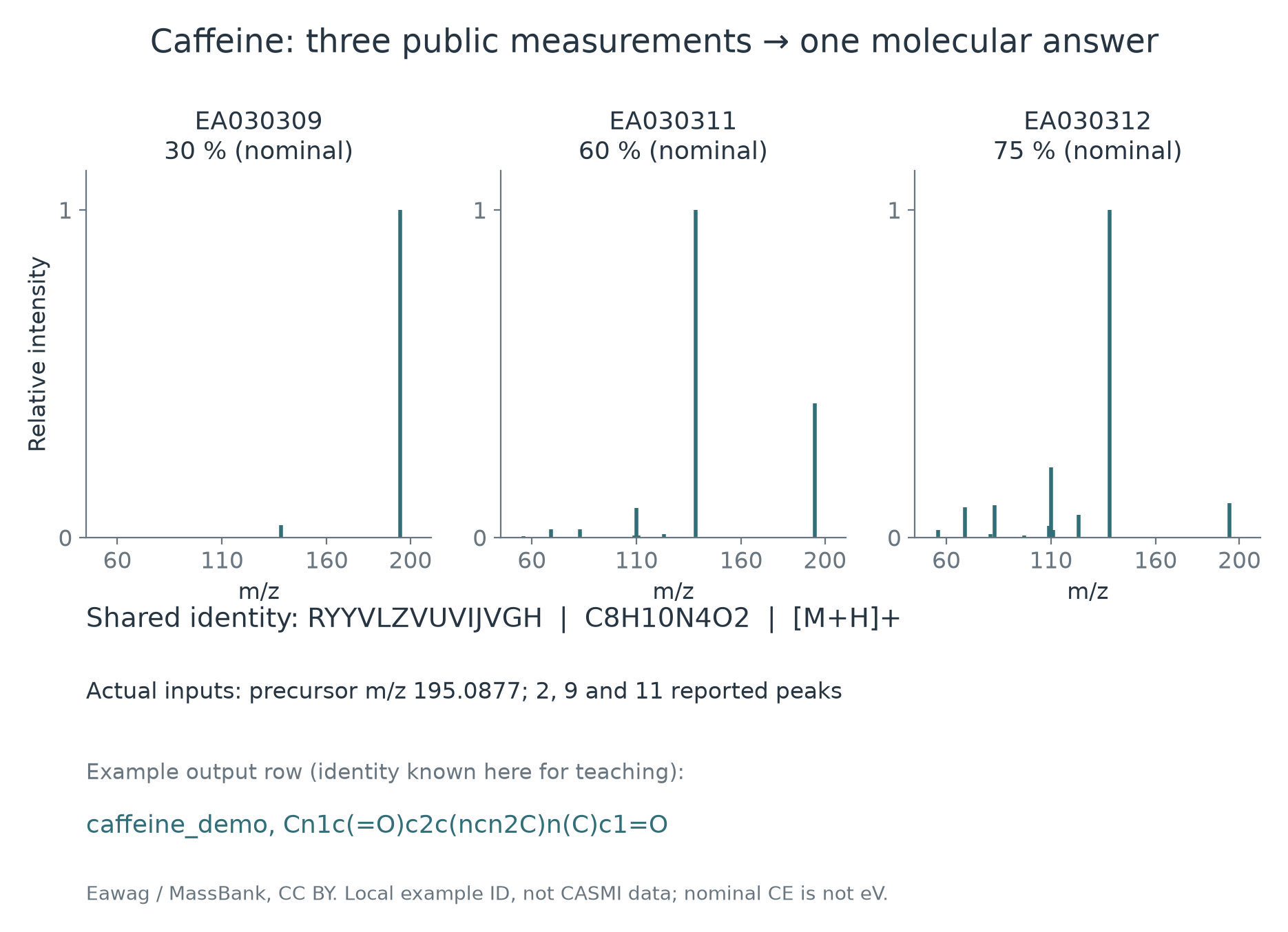
MassBank record	Reported collision energy	Number of listed peaks	Intensity near m/z 195.0877	Intensity near m/z 138.0662	Intensity near m/z 110.0713
EA030309	30% nominal	2	1.0000	0.03693	Not listed
EA030311	60% nominal	9	0.40994	1.0000	0.08968
EA030312	75% nominal	11	0.10565	1.0000	0.21480

Intensities above were recalculated from the original signal values so each spectrum’s base peak is 1. A peak not listed in a processed record is not proof of zero physical abundance. The original records, all peaks, and derivation metadata are available in the shared example JSON.

Here is the complete two-peak record from the 30% measurement, adapted to the relevant CASMI-style fields. The local IDs are illustrative; source_collision_energy is additional provenance, not an official competition column. Percent nominal energy cannot be relabeled as eV, so the eV field remains missing.

example = {
    "molecule_id": "caffeine_demo",
    "spectrum_id": "EA030309",
    "precursor_mz": 195.0877,
    "adduct": "[M+H]+",
    "ionization_mode": "positive",
    "instrument_type": "LC-ESI-ITFT",
    "collision_energy_ev": None,
    "source_collision_energy": "30% nominal",
    "ms2_mzs": [138.0661, 195.0877],
    "ms2_normalized_intensities": [0.0369303417, 1.0],
}

EA030311 and EA030312 would share caffeine_demo but keep their own peak arrays and conditions. An identification procedure must use those three observations to order structures, rather than emit three separate answers. Because Caffeine’s identity is known in this teaching example, one possible illustrative output is:

molecule_id,smiles
caffeine_demo,Cn1c(=O)c2c(ncn2C)n(C)c1=O

For an unknown molecule, the second field contains up to 25 candidates in decreasing confidence, separated by semicolons. The example demonstrates format and grouping, not a model’s identification performance.

Information	Competition columns	Concrete interpretation
Query grouping	molecule_id, spectrum_id	Three Caffeine records become one answer; each observation remains traceable.
Precursor	precursor_mz, adduct	195.0877 with [M+H]+ implies a neutral mass near 194.080424 Da.
Fragment evidence	ms2_mzs, ms2_normalized_intensities	[138.0661, 195.0877] pairs with [0.03693, 1.0].
Conditions	ionization_mode, instrument_type, collision_energy_ev	Preserve polarity and instrument; do not invent an eV conversion.
Training labels and source	normalized_smiles, inchikey, ingest_lib	Identify training structures and audit which libraries supplied their measurements.

Training lacks the test ID columns in the file inspected here; derive training groups from normalized structures. Inspect the actual schema for energy arrays and missing values. Neither a known molecular formula nor a complete MS1 isotope envelope is supplied as a general test input.

Data note: the downloadable test.parquet is a train-derived execution placeholder. Use it for I/O and runtime checks, and a separate molecular holdout for accuracy. Kaggle's public score comes from the hidden evaluation. See the official data description.

2. MRR@25: finding the answer and putting it near the top

The metric is mean reciprocal rank. If the first correct candidate is at rank \(r\), the molecule receives \(1/r\); if no correct answer appears within 25 candidates, it receives zero. Average these contributions over \(U\) molecules. The reference is the official evaluation explanation and implementation.

\[\begin{aligned} \operatorname{MRR@25}&=\frac{1}{U}\sum_{u=1}^{U}\operatorname{RR}_u,\\ \operatorname{RR}_u&=\begin{cases} 1/r_u, & r_u\leq25,\\ 0, & \text{otherwise}. \end{cases} \end{aligned}\]

For example, if four molecules have correct answers at ranks 1, 2, and 5, and outside the list, the score is:

\[\frac{1+0.5+0.2+0}{4}=0.425.\]

This is an illustrative calculation, not a measured result from a model.

Figure 2. A molecule contributes 1 when the correct answer ranks first, 0.5 at rank 2, and 0.04 at rank 25. A change in the overall score is the illustrated contribution change divided by the number of evaluated molecules.

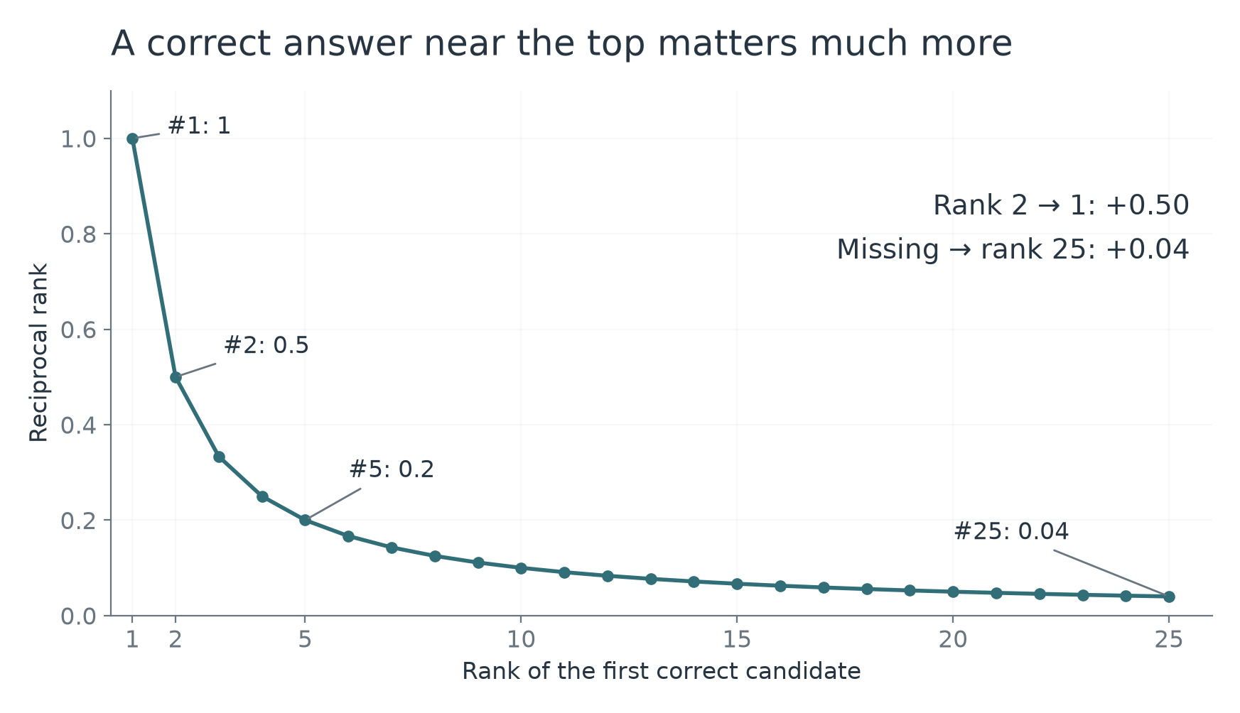
Two properties matter. Finding the answer at rank 25 is better than missing it. Moving an answer from rank 2 to rank 1, however, is worth much more. For one molecule, the first change adds 0.04 and the second adds 0.5: a factor of 12.5.

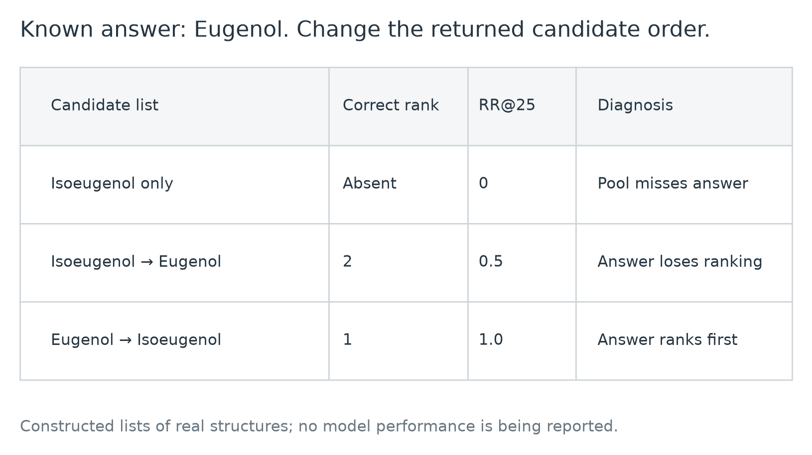
We therefore need to measure whether the answer enters the candidate pool separately from whether the ranking puts it near the top.

Metric	The question it answers
Candidate-pool Recall@K	Is the answer among the K structures passed to the ranker?
Final Hit@25	Is the answer in the 25 submitted candidates?
Top-1 accuracy	Is the first candidate correct?
MRR@25	How often is the answer found, and how early does it appear?

A retrieval pool of K = 1,000 and the final 25 candidates are different stages. If the answer is absent from the pool, the downstream ranker cannot recover it. If Recall@1,000 is high but the correct structure consistently ranks 50th, the final score remains low.

Figure 3. Constructed candidate lists with Eugenol as the known answer. Omitting it gives zero, placing it behind Isoeugenol gives 0.5, and ranking it first gives 1. These lists separate coverage from ordering; they are not model results.

What counts as the same molecule?

The competition uses RDKit 2026.03.3 to canonicalize tautomers, then compares the first 14 characters of the InChIKey. Tautomers are related structural forms that differ in hydrogen placement and bonding. Canonicalization groups forms that the competition treats as equivalent. Using the first InChIKey block also means that stereochemical differences are not distinguished in the final match. Official metric code

This does not mean that matching the molecular formula is enough. Eugenol and Isoeugenol have different keys. The E/Z stereoisomers of Isoeugenol, however, share the connectivity used by this metric. The competition’s answer definition is distinct from complete structural elucidation in a laboratory.

Check it in code: scoring keys and candidate deduplication

The following small example demonstrates the core normalization rule for ordinary single-molecule SMILES. It does not replace the full submission validator or the official scorer’s exception handling.

from rdkit import Chem, rdBase
from rdkit.Chem.MolStandardize import rdMolStandardize

assert rdBase.rdkitVersion == "2026.03.3"
tautomers = rdMolStandardize.TautomerEnumerator()

def scoring_key(smiles):
    mol = Chem.MolFromSmiles(smiles)
    if mol is None:
        raise ValueError(f"Invalid SMILES: {smiles}")
    canonical = tautomers.Canonicalize(mol)
    key = Chem.MolToInchiKey(canonical)
    if not key:
        raise ValueError("InChIKey conversion failed")
    return key[:14]

def unique_candidates(ranked_smiles, limit=25):
    seen, result = set(), []
    for smiles in ranked_smiles:
        key = scoring_key(smiles)
        if key in seen:
            continue
        seen.add(key)
        result.append(smiles)
        if len(result) == limit:
            break
    return result

assert scoring_key("COc1cc(CC=C)ccc1O") != scoring_key("COc1cc(C=CC)ccc1O")
assert scoring_key("C/C=C/c1ccc(O)c(OC)c1") == scoring_key("C/C=C\\c1ccc(O)c(OC)c1")

Generated SMILES that fail parsing should first be recorded and excluded in a separate step. Check that none remain when constructing the final file. Deduplication must preserve the original ranking order.

Candidate coverage sets a ceiling, but does not determine the score

If the final list is drawn only from pool \(C_u\), the empirical score decomposes as

\[\begin{aligned} \operatorname{MRR@25}&=\widehat P(y_u\in C_u)\\ &\quad\times\widehat E\!\left[\frac{\mathbf1\{r_u\leq25\}}{r_u}\;\middle|\;y_u\in C_u\right]. \end{aligned}\]

For example, 80% candidate coverage and conditional mean RR of 0.5 give MRR 0.40. Expanding the database to reach 90% coverage while extra distractors reduce conditional RR to 0.4 gives 0.36. These are calculated values, not project results. Candidate expansion must be evaluated after reranking, with the changed pool reflected in both factors.

3. Three kinds of unknown: remove information one layer at a time

The organizer distinguishes molecules by the information available outside the query. A spectral library pairs measured peaks with known structures; a structure database can contain a molecular graph without any measured spectrum. Class clarification

Type	Correct reference spectrum	Correct structure in public databases	Required ability
Class 1	Available	Known	Match the same structure across measurement conditions.
Class 2	Unavailable	Available	Rank known structures without their own reference spectra.
Class 3	Unavailable	Absent from PubChem and COCONUT	Propose a structure outside those databases.

A controlled Caffeine example

Hold EA030312 (75% nominal CE) as the query. We can change the available evidence while keeping that measured spectrum fixed:

Controlled setting	What the system receives	What success would demonstrate
Class 1-like	Keep EA030309 and EA030311 in the reference library and Caffeine in the candidate pool.	Retrieve Caffeine despite the energy-dependent changes in peak intensities.
Class 2-like	Remove all Caffeine reference spectra and supervised Caffeine examples, but retain its graph among mass-compatible candidates.	Recover the structure using learned fragment/structural evidence or related molecules.
Class 3-like candidate-exclusion test	Also remove Caffeine from every retrieval candidate source.	Generate its graph and place it high enough after candidate deduplication.

Caffeine is a known public molecule, so the third row is a controlled surrogate, not an example of an actual Class 3 test compound. To make the second and third comparisons honest, exclusion must reach all relevant libraries and learned components; deleting two MassBank rows while leaving other Caffeine references would not suffice.

The distinction changes what an experiment can conclude. Perfect ranking on a pool that contains every answer says nothing about generation. Conversely, excluding the answer from a Class 2 pool accidentally tests a harder problem. If a generator requires a molecular formula, that formula must also be inferred from available inputs: supplying the known C8H10N4O2 is an oracle-formula diagnostic, not an end-to-end test.

4. How do we distinguish molecules with the same mass?

Eugenol and Isoeugenol are constitutional isomers with formula \(\mathrm{C}_{10}\mathrm{H}_{12}\mathrm{O}_{2}\) and identical monoisotopic mass. Their side-chain bond connectivity differs. Their structures can be inspected in PubChem’s entries for eugenol and isoeugenol.

Figure 4. The double bond occupies a different position in the two molecules. Structures and masses were calculated from the SMILES below with RDKit 2026.03.3. The 14-character strings are structure keys obtained with the competition's normalization procedure.

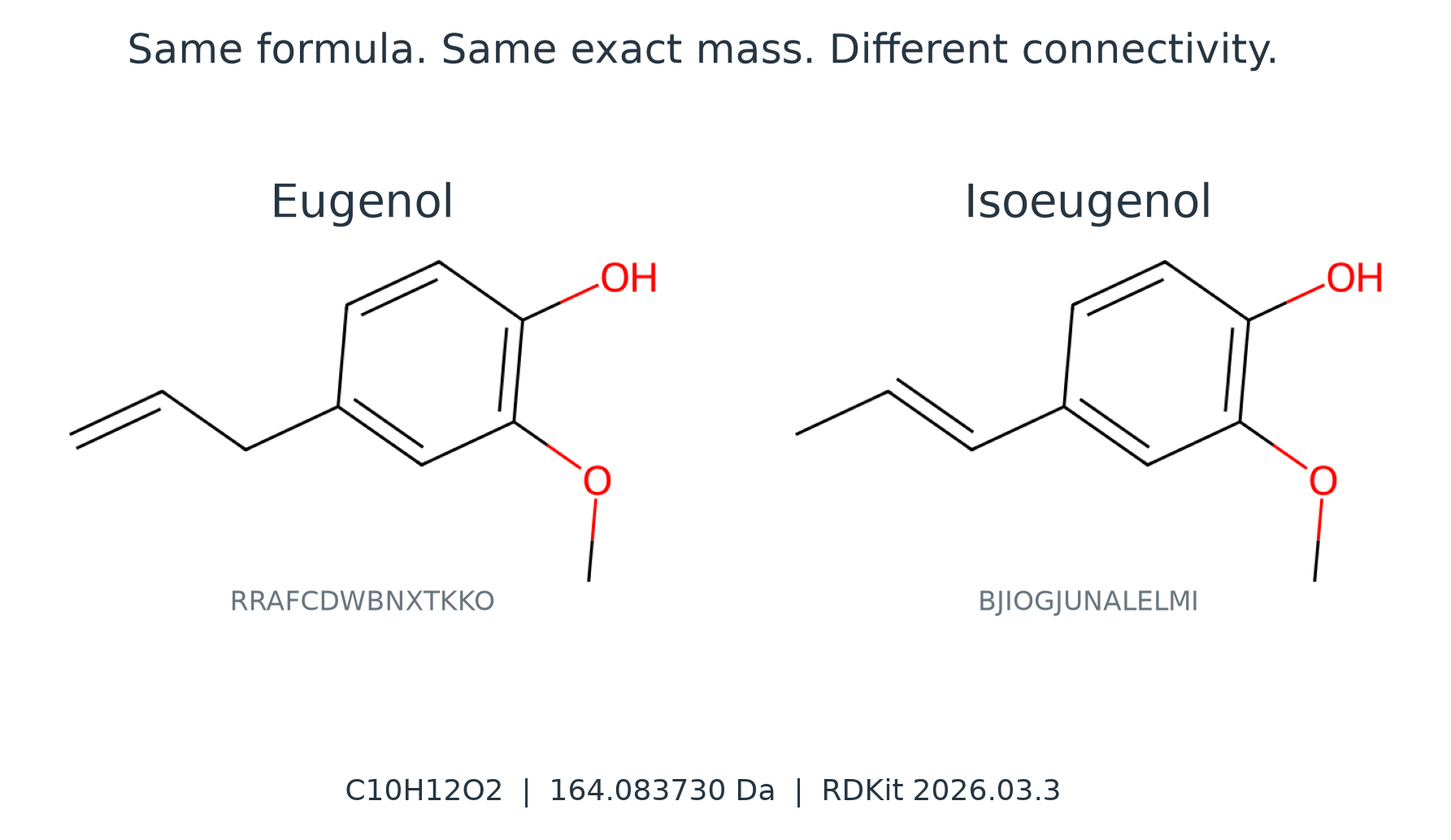
The position of the double bond differs in the three-carbon side chain attached to the ring. These are constitutional isomers: the same atoms connected differently. Knowing that the mass is approximately 164.083730 Da cannot tell us which of the two we have.

This is where fragmentation becomes useful. Different bonding patterns can change where a molecule breaks, where the charge remains, and the relative abundance of the fragments. MS/MS lets us observe such differences. Whether two structures can actually be distinguished depends on the measurement conditions and spectral quality; different structures do not always yield clearly separable spectra.

How do we represent a structure in software?

SMILES encodes a molecular graph as a string. Letters represent atoms, while symbols describe bonds, branches, and ring closures. Our two examples can be written as follows.

Eugenol:     COc1cc(CC=C)ccc1O
Isoeugenol:  COc1cc(C=CC)ccc1O

The lowercase c denotes aromatic carbon, = denotes a double bond, and parentheses indicate branches. We do not need to memorize the entire syntax to begin. The target of the competition is the molecular structure represented by the string.

The same molecule can have different SMILES strings depending on where traversal begins. Comparing prediction and target strings directly would therefore be wrong. The competition normalizes structures before comparing them, as explained in Section 2.

The following code calculates the formulas and masses of both examples. RDKit is an open-source toolkit widely used to read and work with molecular structures.

from rdkit import Chem
from rdkit.Chem import Descriptors, rdMolDescriptors

structures = {
    "Eugenol": "COc1cc(CC=C)ccc1O",
    "Isoeugenol": "COc1cc(C=CC)ccc1O",
}

for name, smiles in structures.items():
    mol = Chem.MolFromSmiles(smiles)
    print(name, rdMolDescriptors.CalcMolFormula(mol),
          f"{Descriptors.ExactMolWt(mol):.6f}")

Eugenol C10H12O2 164.083730
Isoeugenol C10H12O2 164.083730

These values differ from the average molecular weight commonly shown in a composition table. Exact mass is calculated for a specified isotopic composition. Here we calculate monoisotopic mass, using the most abundant isotope of each element. This is the relevant quantity when working with small mass differences in high-resolution mass spectrometry.

Why calculate so many decimal places?

The number of protons in a nucleus determines its element. Atoms of the same element with different neutron counts are isotopes. The mass of \(^{12}\mathrm C\) is exactly 12 Da, whereas \(^1\mathrm H\) and \(^{16}\mathrm O\) have masses of approximately 1.007825 and 15.994915 Da. Adding integer atomic masses would discard these differences. The values come from the NIST tables for carbon, hydrogen, and oxygen.

For a specified isotopic composition, molecular mass is calculated by summing atomic masses. At the precision used here, the extremely small mass difference associated with chemical binding energy is neglected.

\[m_{\mathrm{exact}}=\sum_e n_e\,m_e.\]

Here, \(n_e\) is the atom count and \(m_e\) is the mass of the selected isotope. For Eugenol, this gives:

\[\begin{aligned} m&=10(12)+12(1.007825032)\\ &\quad+2(15.994914620)\\ &\simeq164.083730\ \mathrm{Da}. \end{aligned}\]

Two formulas with different atom counts can share the same integer mass and still differ in their decimal places. Eugenol and Isoeugenol, however, have the same formula and cannot be separated this way, regardless of mass accuracy. More accurate mass measurements constrain composition; they do not directly reveal the order in which atoms are connected.

Isotopes also produce additional spectral peaks. Replacing one \(^{12}\mathrm C\) atom with \(^{13}\mathrm C\) adds approximately 1.003355 Da. For ions with the same charge number \(z\), the corresponding separation in \(m/z\) is:

\[\Delta(m/z)\simeq\frac{1.003355}{|z|}.\]

A sufficiently informative isotope pattern can help constrain charge and elemental composition. However, the CASMI input does not provide a complete MS1 isotope envelope as a separate array. Information that is useful in mass spectrometry generally should not be assumed to exist in the competition files. Any use of isotope-related peaks remaining in MS2 lists must account for how those lists were processed.

What can a formula tell us? Valence and unsaturation

Matching the mass is not sufficient when proposing a formula. For ordinary organic molecules, we usually begin with the familiar valences of carbon, oxygen, and neutral nitrogen: four, two, and three bonds, respectively. These constraints mean that an arbitrary combination of atom counts need not correspond to a valid molecular graph.

A useful example is the degree of unsaturation, or double-bond equivalent (DBE). For neutral, closed-shell C/H/N/O/halogen molecules with conventional valences, we can write:

\[\operatorname{DBE}=1+C-\frac{H+X}{2}+\frac{N}{2}.\]

The letters denote atom counts; \(X\) is the total number of halogen atoms such as F, Cl, Br, and I. Divalent oxygen does not appear explicitly in this expression. Relative to a saturated acyclic hydrocarbon, removing two hydrogens allows one ring or one double bond; a triple bond counts as two units.

For Eugenol, \(1+10-12/2=5\). The benzene ring contributes four units—one ring and three double bonds—and the side-chain double bond contributes one. Isoeugenol has the same DBE. The quantity constrains possible structures but does not rank these two isomers.

In CASMI, this knowledge can help check formulas and generated candidates. It should not become a universal rejection rule for all ions and elements. Charge, radicals, and the multiple valence states of phosphorus and sulfur complicate the interpretation. Kind and Fiehn’s original work on formula filtering discusses these limitations. Any chemical constraint needs a stated scope and a check on how often it incorrectly removes the true candidate.

5. From measured peaks to a physical model

LC separates a mixture, ionization produces gas-phase ions, and a selected precursor fragments before its products are measured. CASMI starts from processed MS/MS peak lists, not raw chromatograms. A spectrum is a sparse pair of arrays: calibrated m/z and detected relative intensity.

Figure 5. All 11 listed peaks in EA030312. The base peak is m/z 138.0662; 110.0713 and the residual precursor at 195.0878 have relative intensities 0.21480 and 0.10565. Source: Stravs, Schymanski and Singer, Eawag/MassBank, CC BY.

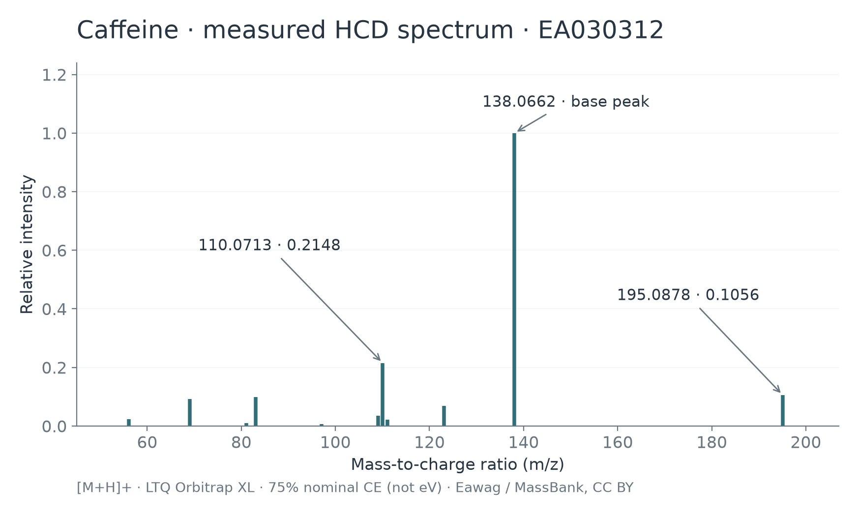
For example, the full 30% Caffeine record contains ms2_mzs = [138.0661, 195.0877] and normalized intensities [0.0369303417, 1.0]; the 75% record in Figure 5 has eleven peaks. The strongest is the base peak. Array positions pair masses and intensities, but neither the peak count nor a maximum intensity of 1 measures identification certainty. The relevant physics explains which information survives this representation and which conditions alter it.

How does an instrument read mass?

The timsTOF instrument family used in the competition combines trapped ion mobility with quadrupole time-of-flight mass spectrometry. The basic idea behind time of flight (TOF) is to measure how long an accelerated ion takes to travel a specified distance. Bruker’s instrument overview

In an idealized model, an ion with negligible initial kinetic energy is accelerated through a potential difference \(V\). Conservation of energy gives:

\[\begin{aligned} |z|eV&=\frac12m_{\mathrm{ion}}v^2,\\ t&=\frac Lv=L\sqrt{\frac{m_{\mathrm{ion}}}{2|z|eV}}. \end{aligned}\]

Here, \(e\) is the elementary charge, \(v\) is velocity, and \(L\) is the flight distance. Use SI units in this equation: kilograms for mass, volts for potential difference, and meters for distance. For the same potential difference and path, flight time scales with the square root of the mass-to-charge ratio. Arrival times can therefore be converted into calibrated \(m/z\) values. Real instruments include more elaborate corrections for energy distributions and flight paths.

We receive peak positions that have already undergone this conversion. Nor should the presence of ion mobility hardware lead us to assume that collision cross section (CCS) or mobility time is supplied as an input. What an instrument can measure and what the dataset actually contains are separate questions.

Keep the physical quantities and their units distinct.

Quantity	Meaning and units	What to distinguish here
Neutral exact mass	Mass calculated from isotopic composition, in Da	The neutral molecule before ionization
Charge number z	Signed integer multiple of elementary charge	Divide by its magnitude |z| when calculating m/z
Spectral m/z	Ion mass divided by charge-number magnitude	Converting to neutral mass requires the adduct and charge
Collision energy	A collision condition, expressed in eV or other conventions	Distinguish instrument voltage, NCE, and actual internal energy
Molar activation energy	Reaction barrier expressed per mole, for example kJ/mol	Match the units of R in the Arrhenius equation
Relative intensity	Normalized signal within one spectrum, dimensionless	It does not give an absolute abundance ratio across spectra

For a numerical scale, an idealized singly charged 195 Da ion accelerated through 5,000 V over a 1 m path takes about 14.22 μs. Doubling the ion mass increases that time by a factor of √2. These are chosen geometry/voltage values, not timsTOF operating specifications. CASMI already supplies calibrated m/z, so a model needs mass-error handling rather than a flight-time simulator.

Precursor m/z is not the neutral molecular mass

A mass analyzer uses electric fields to move and separate ions. The relevant question is therefore which ionic form enters the instrument. Electrospray ionization (ESI), widely used in LC-MS, forms gas-phase ions through processes involving charged droplets and solvent removal. It is sufficiently gentle to preserve intact molecular ions in many cases, but molecules differ in ionization efficiency and in the ionic forms they produce. Agilent’s LC/MS introduction

For example, [M+H]+ is a neutral molecule \(M\) with an added proton. [M-H]- has lost a proton, while [M+Na]+ carries a sodium ion. The dataset describes these ionic forms through its adduct information. Solution acidity, functional groups, solvents, and salts can affect which forms are observed. Technical explanation of LC conditions and ionization

Let the signed mass change on forming the ion be \(\Delta m_{\mathrm{ion}}\). Using masses in Da, we can write:

\[\begin{aligned} (m/z)_{\mathrm{precursor}} &=\frac{m(M)+\Delta m_{\mathrm{ion}}}{|z|},\\ m(M)&=|z|(m/z)_{\mathrm{precursor}}-\Delta m_{\mathrm{ion}}. \end{aligned}\]

Several examples for singly charged ions make the conversion concrete.

Ionic form	Mass change relative to the neutral, \(\Delta m_{\mathrm{ion}}\)	Recovering neutral mass
[M+H]+	Approximately +1.007276 Da	Subtract 1.007276 from precursor m/z
[M-H]-	Approximately −1.007276 Da	Add 1.007276 to precursor m/z
[M+Na]+	Approximately +22.989221 Da	Subtract 22.989221 from precursor m/z
[M-H2O+H]+	Approximately −17.003288 Da	Add 17.003288 to precursor m/z

If Eugenol is observed as [M+H]+, its precursor m/z is approximately 165.091006. Treating that as the neutral mass would cause retrieval to miss the answer. The 1.007276 in the table is also the proton mass, not the neutral hydrogen-atom mass of 1.007825. Their difference is approximately one electron mass, 0.000549 Da, or about 3.3 ppm near 164 Da. That matters for a narrow mass window. These are mass-calculation conventions, not instructions to apply a blanket correction to measured peaks.

Thus even the first step of finding nearby masses requires adduct interpretation. The data description covers positive and negative ions and water-loss forms; an update announcement also describes corrected water-loss annotations in the training data.

The Caffeine precursor gives a direct check: 195.0877 − 1.0072764666 = 194.0804235334 Da, consistent with the source’s rounded neutral exact mass of 194.0804. A 5 ppm neutral-mass window here is about ±0.0009704 Da. Misreading the adduct as [M+Na]+ instead shifts the inferred neutral mass by nearly 22 Da; increasing a ppm tolerance cannot repair that categorical error.

Where the proton sits can change fragmentation

The notation [M+H]+ tells us that a proton has been added, but does not specify its location. Molecules with several nitrogen or oxygen atoms can have multiple protonation sites, and the proton can move during fragmentation. Charge location changes electron distribution and the pathways available for dissociation. A CIDMD study of small molecules examines why this matters for spectrum prediction.

This also brings in resonance and conjugation. Delocalizing charge over several atoms can stabilize a fragment ion. The existence of a stable fragment, however, does not guarantee a pathway that produces much of it within the observation time.

For CASMI, ignoring polarity and adducts would combine different physical processes into one target spectrum for the same neutral structure. A structure-to-spectrum model should use the available measurement conditions, and its limitations should be checked for adducts outside its training support. Solution-phase acidity alone is also insufficient to determine the protonation site of a gas-phase ion.

For a candidate with two plausible protomers, a conditional spectrum model could represent the observation as a mixture, \(p(s\mid c,\theta)=\sum_h p(s\mid c,h,\theta)p(h\mid c,\theta)\), where \(h\) indexes protonation states. If two protomers emphasize different fragments, replacing them by one arbitrary protonation site can create a systematic residual. This is a modeling interpretation, not an assertion that the public FPNet explicitly enumerates protomers. In practice, begin by separating supported positive/negative adduct conditions and inspecting their held-out errors.

Collision energy is not energy deposited directly into one bond

In collision-induced dissociation (CID), an ion collides with neutral gas and converts part of its translational kinetic energy into internal energy, which can lead to fragmentation. Internal energy includes molecular vibration. This is the process described by IUPAC’s definition of CID.

A collision energy of 30 eV does not mean that 30 eV has been placed into one bond. Consider the simplest case: an ion colliding with a stationary gas particle. The ion’s kinetic energy in the laboratory frame, \(E_{\mathrm{lab}}\), and the relative-motion energy available in the center-of-mass frame, \(E_{\mathrm{cm}}\), are related by:

\[E_{\mathrm{cm}} =\frac{m_{\mathrm{gas}}}{m_{\mathrm{ion}}+m_{\mathrm{gas}}} E_{\mathrm{lab}}.\]

The relationship follows by subtracting the kinetic energy of the overall center-of-mass motion from the two-body kinetic energy. As an illustrative calculation, a 300 Da ion colliding with a 28 Da gas particle at \(E_{\mathrm{lab}}=30\) eV gives \(E_{\mathrm{cm}}\simeq2.56\) eV. For a 1,000 Da ion, the value is about 0.82 eV. Even this energy is not all deposited into the ion’s internal modes. Actual experiments also depend on collision counts, gas, residence time, and energy distributions. The MassKinetics study connects energy transfer with reaction rates.

Here, \(E_{\mathrm{lab}}\) means the total kinetic energy of the ion. If an instrument reports acceleration voltage or normalized collision energy instead, its definition must be checked first. Substituting the competition’s collision_energy_ev into this equation does not directly reconstruct actual internal energy.

The same 20 eV label on different instruments therefore need not describe identical physical conditions. Collision energy is a useful input, but it should be interpreted with instrument and ion information. Filling missing energy values with zero would also confuse an unknown measurement with the absence of supplied energy.

Our measured records make the units issue concrete: 30%, 60%, and 75% nominal HCD energy are source settings, not 30, 60, and 75 eV. They support within-series comparison on the same instrument; they cannot calibrate the hidden timsTOF energy scale by numerical equality. A condition encoder should distinguish unit convention and missingness, or use a checkpoint’s documented preprocessing when that metadata cannot be supplied.

Which fragments become abundant? Stability and reaction rates

Single bond-cut enumeration cannot reproduce an ion spectrum: a fragmentation pathway must cross an activation barrier and proceed within the observation time. Some pathways involve hydrogen transfer or structural rearrangement. Average bond dissociation energies for neutral molecules cannot simply rank all possible dissociation routes of an ion.

Figure 6. Analytic populations for kA = 3,000 s⁻¹ and kB = 1,000 s⁻¹, starting from P = 1. Rates are fixed and products do not react further. This numerical example is not fitted to Caffeine or any experimental spectrum.

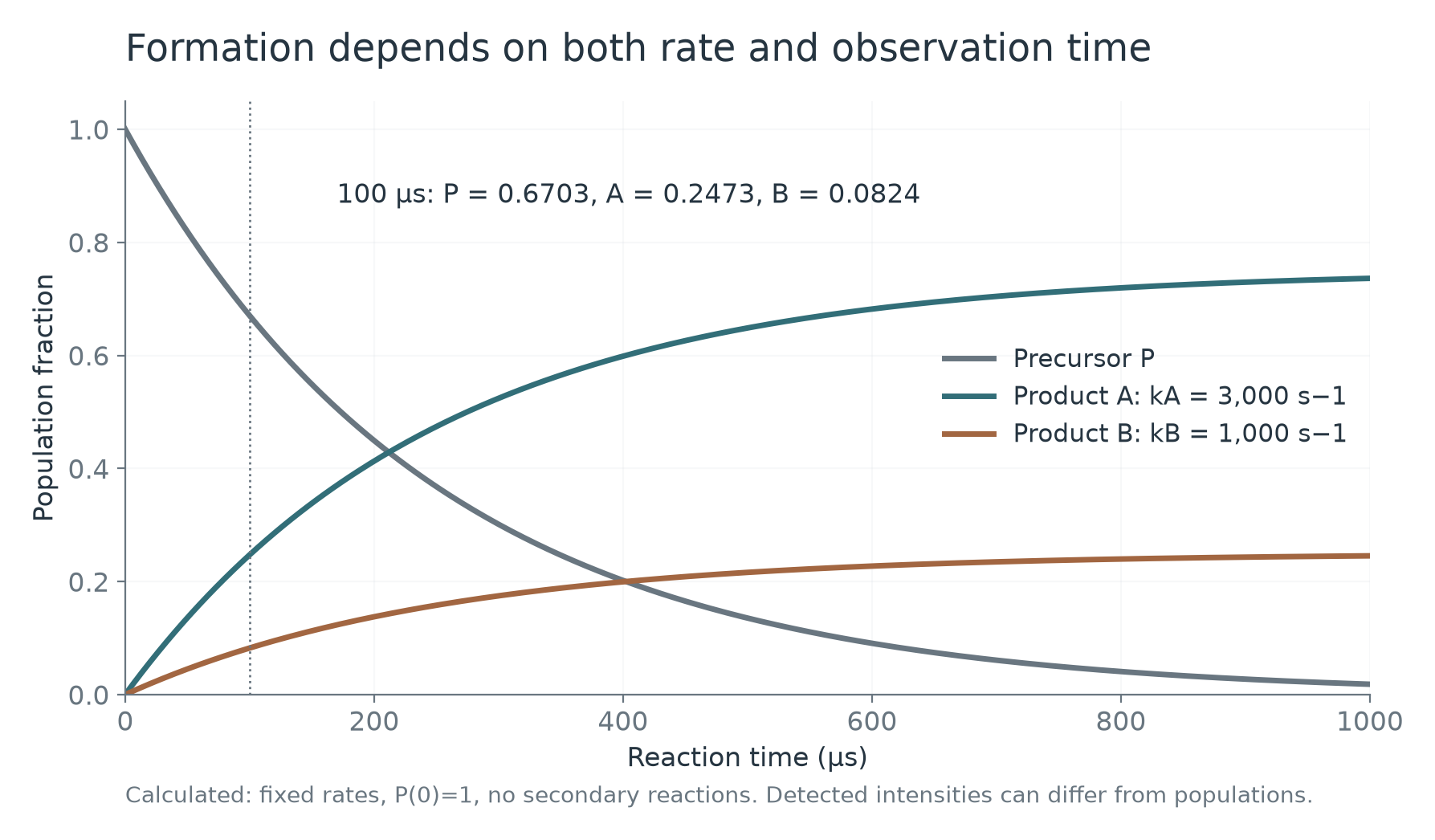
A simple kinetic example has two competing pathways from an excited precursor ion \(P^{+*}\):

\[P^{+*}\xrightarrow{k_A}A^++N_A, \qquad P^{+*}\xrightarrow{k_B}B^++N_B.\]

Here, \(N_A,N_B\) are undetected neutral products, and \(k_A,k_B\) are the rate constants. If these are the only reactions, both rate constants are fixed, and the products do not fragment further, the fraction of precursors that has reacted is:

\[f_{\mathrm{reacted}}(t)=1-e^{-(k_A+k_B)t}.\]

The fractions of product ions entering paths A and B are \(k_A/(k_A+k_B)\) and \(k_B/(k_A+k_B)\). If A proceeds three times as fast as B, this simple model gives a 3:1 formation ratio. The measured intensity ratio is not necessarily 3:1. Different transmission or detection efficiencies, or subsequent fragmentation, can change it.

Even this small model gives us a reason to predict peak presence and intensity separately. Knowing which fragments are possible differs from knowing how much of each will form and survive. Separating fragment generation from intensity prediction in a forward model can be understood in this way.

A closer look: the Arrhenius equation and RRKM theory

An introductory treatment of reaction kinetics often begins with the Arrhenius equation:

\[k(T)=A\exp\!\left(-\frac{E_a}{RT}\right).\]

Here, \(E_a\) is the molar activation energy, \(R\) is the gas constant, and \(T\) is temperature. The equation helps explain the relationship between barriers and rates. However, a mass spectrometer’s collision-energy setting cannot simply be substituted for \(RT\). An ensemble’s internal-energy distribution is not the same input as a thermal-equilibrium temperature.

RRKM theory is a statistical framework for unimolecular reactions of ions at a fixed internal energy \(E\). Its basic form is:

\[k(E)=\frac{N^{\ddagger}(E-E_0)}{h\rho(E)}.\]

Here, \(E_0\) is the threshold energy, \(\rho(E)\) is the reactant density of states, \(N^{\ddagger}\) is the number of transition-state states accessible at the available energy, and \(h\) is Planck’s constant. Assumptions about statistical energy redistribution are required, and not all fragmentation follows this model. A study estimating gas-phase ion dissociation energies provides an application.

There is no need to implement an RRKM calculator before entering CASMI. The useful implication is that dissociation rates depend on the states and internal energy of the whole molecule, not only on the energy of one bond. A matching fragment mass alone cannot determine its intensity.

Put numbers into the two-pathway example: \(k_A=3{,}000\ \mathrm{s}^{-1}\) and \(k_B=1{,}000\ \mathrm{s}^{-1}\). At 100 μs, the precursor fraction is 0.6703, while A and B contain 0.2473 and 0.08242 of the initial population. At 1 ms these become 0.01832, 0.7363, and 0.2454. If A’s transmission/detection factor is 0.5 and B’s is 1, their detected ratio is 1.5 rather than their formation ratio of 3. This is an analytic example with fixed rates and no secondary reactions, not a fit to Caffeine. It explains why instrument response and reaction time belong in interpreting an intensity target.

Neutral losses: reading an undetected fragment from a mass difference

When an ion fragments into a charged product and a neutral product, the charged product is normally the one detected. The mass difference between precursor and product can therefore provide evidence about the neutral loss.

For a pathway that loses one neutral molecule while retaining the same single charge:

\[m_{\mathrm{loss}} \simeq(m/z)_{\mathrm{precursor}}-(m/z)_{\mathrm{fragment}}.\]

If the two ions have the same charge magnitude but \(\lvert z\rvert>1\), multiply the separation by \(\lvert z\rvert\). If the charge changes or other reactions intervene, simple subtraction does not support the same interpretation.

Example neutral species	Monoisotopic mass	A question to ask
Water, H₂O	Approximately 18.010565 Da	Does the composition and pathway allow dehydration?
Ammonia, NH₃	Approximately 17.026549 Da	Can the structure account for this nitrogen- and hydrogen-containing loss?
Carbon monoxide, CO	Approximately 27.994915 Da	Is there a plausible pathway for losing this composition?
Carbon dioxide, CO₂	Approximately 43.989829 Da	Can the structure support decarboxylation or another route to this loss?

These numbers are calculated masses for neutral compositions. A pair of peaks separated by about 18.010565 Da does not establish the presence of an OH group at a particular position. Water can form through hydrogen transfers and rearrangements involving multiple atoms. Conversely, an OH-containing structure need not show an appreciable water-loss peak under every condition.

In CASMI, we can compare neutral-loss lists alongside fragment \(m/z\) lists, or calculate the fraction of peaks that a candidate’s elemental composition can explain. These are useful features to test with other evidence before turning them into hard rejection rules. Mass calculations use the NIST tables above and the nitrogen isotope table.

Figure 7. Measured peak separations in EA030312 and calculated neutral masses. The ion formulas are tentative annotations from the source. Agreement in composition does not establish sequential fragmentation or identify the atoms lost.

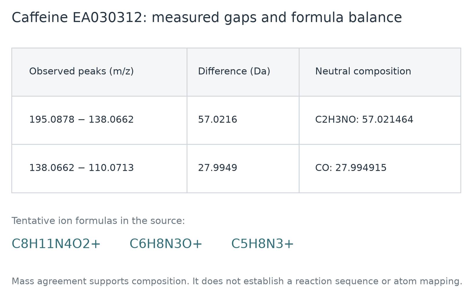
Now use the measured EA030312 peaks. The source tentatively assigns 138.0662 to C6H8N3O+ and 110.0713 to C5H8N3+. Their difference is 27.9949 Da, agreeing with the calculated CO mass 27.994915 Da. The residual precursor peak at 195.0878 minus 138.0662 gives 57.0216 Da, consistent with neutral C2H3NO at 57.021464 Da and with the source’s tentative ion formulas. The selected-precursor metadata are 195.0877; using those instead gives 57.0215, so we must specify which value is subtracted. Measured record and tentative annotations

These agreements constrain elemental bookkeeping. They do not show that 195 → 138 → 110 is a sequential mechanism, locate the departing atoms, or exclude rearrangements. A model can use both peak-pair residuals as features without pretending they are proved reaction edges.

Resolving power and mass accuracy describe different properties

Mass resolving power describes the ability to separate nearby peaks. With peak width defined as the full width at half maximum (FWHM), the expression is: IUPAC definition

\[R=\frac{m}{\Delta m_{\mathrm{FWHM}}}.\]

Mass accuracy, by contrast, concerns how close the measured peak center is to its true value. A narrow peak can still be shifted. High resolving power is therefore not, by itself, a reason to make a retrieval tolerance extremely narrow.

CASMI’s ms2_mzs contains peak locations, not a raw peak profile and FWHM for every peak. Many decimal places do not establish measured resolving power. When comparing libraries, use available labeled data to examine precursor and fragment error distributions separately and choose matching tolerances accordingly.

At m/z 200, \(R=30{,}000\) corresponds to a 0.00667 FWHM, whereas a 5 ppm centroid error is 0.00100. One number describes a peak’s width, the other its displacement. Similarly, fixed 0.01-wide bins can merge distinct nearby peaks; a sparse peak matcher can retain their exact positions. Choose resolution and tolerance from the processing task and measured error distributions, rather than equating decimal precision with instrument resolution.

Different collision energies ask different questions about the structure

At lower energies, a molecule may retain more precursor and larger fragment ions. At higher energies, further dissociation can produce smaller fragments. An intermediate fragment can first become more abundant and then decline as it fragments again.

Figure 8. EA030309, EA030311 and EA030312 from the same LTQ Orbitrap XL series. Each record is normalized independently; vertical values compare relative spectral shapes, not total ion abundance. Eawag/MassBank, CC BY.

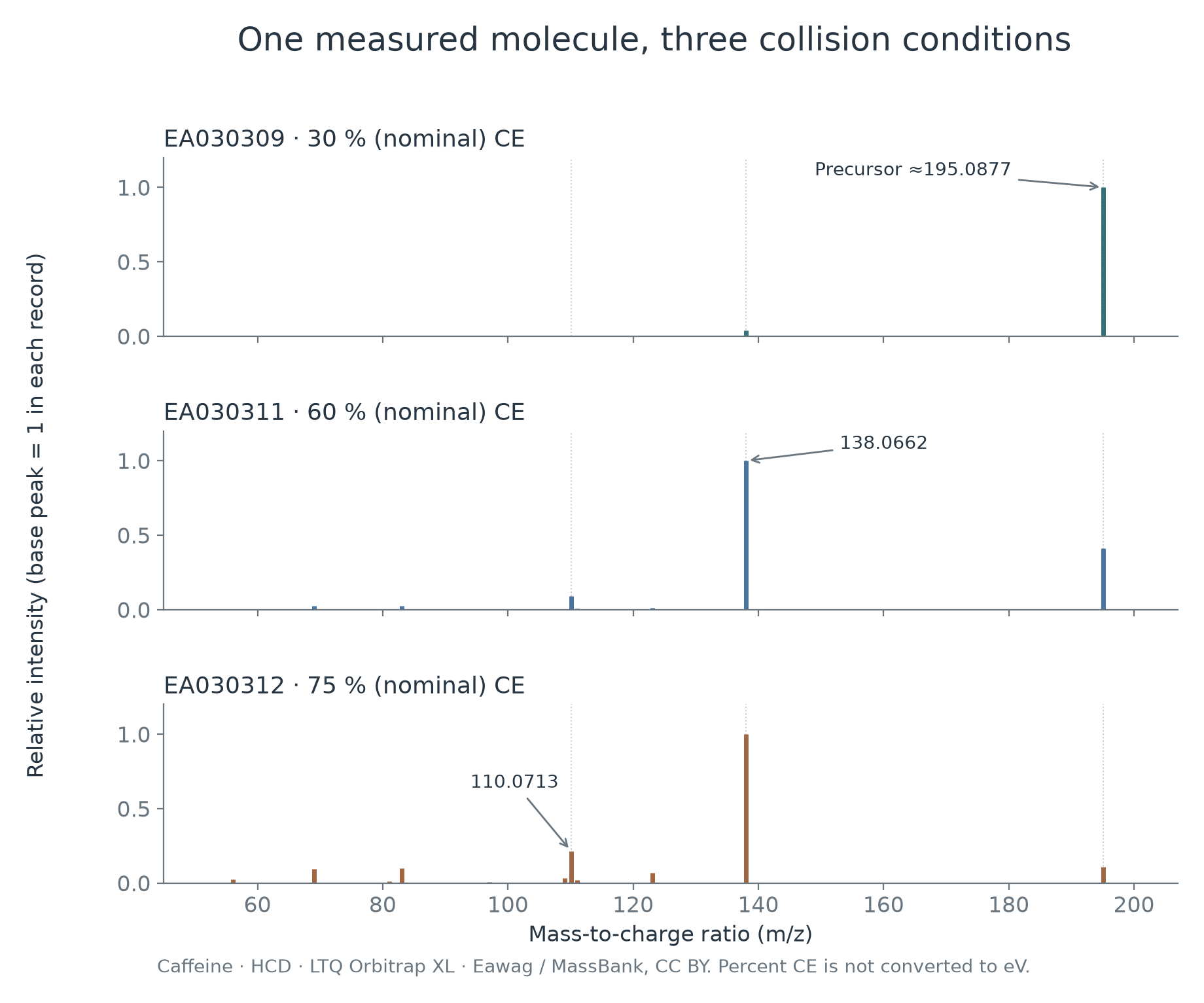
A candidate that explains large fragments at low energy may differ from one that explains smaller fragments at high energy. Agreement across conditions can provide stronger evidence. However, treating nearly duplicate spectra from similar conditions as independent evidence can exaggerate confidence.

Intensity normalization also matters. The competition’s base-peak normalization can be written as:

\[\widetilde I_i=\frac{I_i}{\max_j I_j}.\]

This preserves the relative shape within a spectrum but removes the absolute intensity scale. Even when base_peak_intensity is supplied separately, it cannot directly represent concentration or prediction confidence without accounting for amplification, ionization efficiency, injection amount, and other effects. Both a sparse spectrum and a rich spectrum can have a maximum normalized peak of 1.

In the actual series, the 138 peak changes from 0.03693 → 1.0000 → 1.0000, the residual precursor from 1.0000 → 0.40994 → 0.10565, and the 110 peak from unlisted → 0.08968 → 0.21480. These are separately normalized relative signals, not ion yields. The 30% record mainly constrains precursor survival and one fragment; the 75% record contains 11 listed peaks and more fragment evidence. A merged spectrum loses that distinction unless energy-specific observations remain available.

For aggregation, compare a mean over spectra with a mean over distinct condition groups. If one condition has ten near-duplicate measurements and another only one, an unweighted row mean gives the first condition ten times the influence. That may reflect sampling frequency rather than ten independent pieces of structural evidence.

Turning the background into a prediction problem

Let \(c\) be the unknown structure, \(\mathcal S\) the collection of spectra, and \(\Theta\) the measurement conditions. Identification can be viewed as an inverse problem:

\[p(c\mid\mathcal S,\Theta) \propto p(\mathcal S\mid c,\Theta)\,p(c\mid\Theta).\]

The first term on the right asks whether a structure could plausibly produce the measurements. The second describes its plausibility before considering those measurements. This is a conceptual framework, not the official scoring formula.

A forward model supplies evidence related to the first question. Spectral libraries and structure databases determine which candidates we compare. Preference for structures common in training can also introduce a bias resembling the second term. Validation should help distinguish explaining a spectrum from merely preferring a familiar candidate.

The Bayesian view also clarifies a concrete ambiguity. Eugenol and Isoeugenol pass the same exact-mass constraint; that constraint cannot change their relative odds. A fragment-pattern score can change the likelihood ratio, while a database-frequency feature changes a prior-like preference. On a source-shifted natural-product panel, the latter may fail even if the mass is perfect. Test this with an ablation on the same candidates, then examine which same-formula pairs change order.

The input columns now have a physical meaning: they contain evidence gathered under particular conditions. Next we examine which molecules and instruments the training data cover, then connect that evidence to candidate retrieval and ranking.

6. What is inside 2.5 million training spectra?

The official description gives approximately 2.5 million spectra and 275,000 structures, combining public libraries with Enveda data. Competition data

The local file audited for this project contained 2,539,608 rows and 275,810 structures according to the supplied structure keys. That structure count is an aggregation of the keys already in the file. It should not be assumed to equal a count obtained after rerunning the metric’s normalization on every structure.

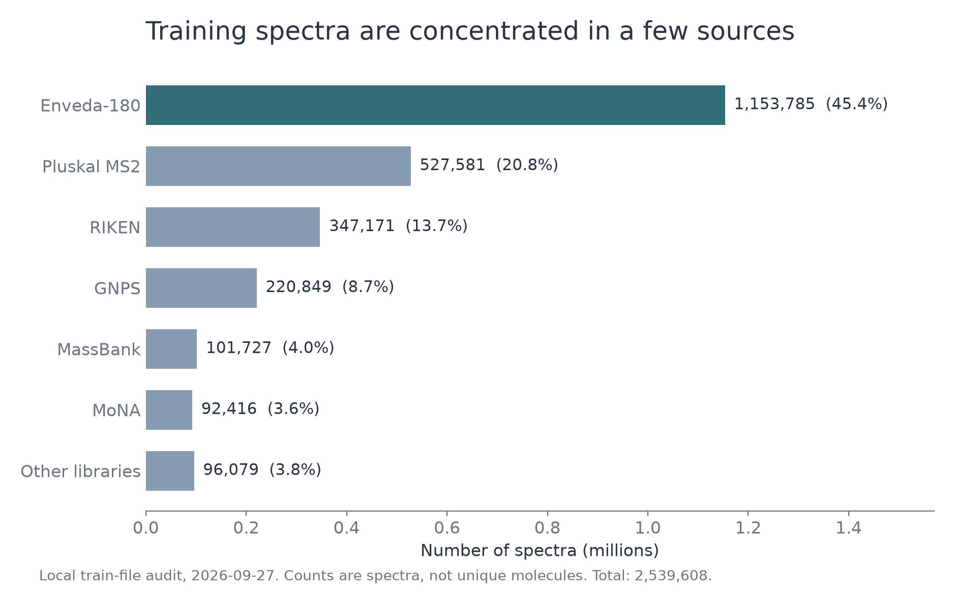
Figure 9. Aggregation of ingest_lib in the local training file on September 27, 2026. Bars count spectra, not molecules. The Other libraries group combines SpectraVerse, MS-DIAL, drug_plus, natural-product examples, and Masaryk data.

Enveda-180 is the largest source: approximately 1.15 million spectra, or about 45% of the total. Enveda’s public processing code provides useful context for its construction and processing.

A large row count does not automatically imply sufficient information about the target molecules. A structure can be measured at multiple collision energies, and sources differ in both chemistry and instrumentation. One hundred spectra from one hundred molecules carry different information from one hundred spectra covering only ten molecules.

Matching the instrument does not guarantee matching the chemistry

Enveda data are attractive because the hidden test is measured on timsTOF. However, a substantial part of Enveda-180 covers synthetic compounds, whose structural distribution need not match the natural products and analogs of interest here. Other libraries can add natural-product diversity while differing in instruments and collision-energy conditions.

We need to consider both:

• Measurement shift: the same structure can produce different spectra across instruments, energies, and adducts.
• Chemical-space shift: unfamiliar scaffolds and substructures can appear even when the instrument is unchanged.

Weighting every library in proportion to its row count can let the largest source dominate training. Repeating only a small natural-product subset can instead encourage overfitting. Sampling by molecule and source is worth testing, but its effect must be established through structure-level validation.

The training file has two roles. Its measured spectra paired with known structures are immediately useful as search references, and those same pairs can train a model of the relationship between spectra and structures. This is why retrieval is a sensible first step even when a large training set is available.

Match the training weight to the evaluation unit

Suppose one molecule contributes 20 spectra and another contributes 2. A row-averaged loss gives the first ten times the total weight, while MRR gives each molecule one vote. One possible correction is

\[\mathcal L=\frac1U\sum_{u=1}^{U}\frac1{n_u}\sum_{i=1}^{n_u}\ell(s_{ui},y_u).\]

This weights molecules equally while averaging their observations. Source balancing is an additional choice: equal molecule weights do not make chemical coverage or instrument coverage equal. Compare row sampling, molecule sampling, and source-stratified molecule sampling on the same held-out groups, and report both aggregate MRR and the timsTOF/natural-product-relevant subgroups. The source counts in Figure 9 describe sampling pressure; they do not establish the best weighting.

7. Build the candidate pool through retrieval and analogs

Library search is a straightforward starting point. Compare the query with reference spectra of known structures, then retrieve the structures associated with similar measurements.

Match peaks before calculating similarity

A simple approach matches peaks at nearby \(m/z\) values and calculates cosine similarity. For aligned intensity vectors \(x,y\):

\[\operatorname{cosine}(x,y) =\frac{x\cdot y}{\lVert x\rVert_2\lVert y\rVert_2}.\]

Peak positions will rarely coincide exactly, so matching within a tolerance comes first. We can also take square roots of intensities to reduce the dominance of large peaks, or compare neutral losses, the mass differences from precursor to fragment. The Fast Spectral Cosine baseline and matchms are useful implementation references.

The method is interpretable: a reference spectrum can explain why a structure was retrieved. Its limitation is equally clear. If no spectrum of the correct structure exists in the library, direct same-structure retrieval cannot return it.

Narrowing structure candidates by mass

This is where structure databases such as COCONUT and PubChem become useful. Estimate neutral mass from precursor m/z and adduct, then collect structures within a tolerance.

Mass error in parts per million is:

\[\operatorname{ppm\ error} =10^6\frac{m_{\mathrm{candidate}}-m_{\mathrm{query}}}{m_{\mathrm{query}}}.\]

At 164.083730 Da, ±10 ppm corresponds to approximately ±0.001641 Da. This illustrates the scale of a mass tolerance; it is not a recommended optimum for this competition. A window that is too narrow can discard the answer because of measurement error or incorrect adduct handling. A wide window increases candidate counts and computation.

Passing the mass filter makes a structure eligible for comparison; it does not identify it. Isomers such as Eugenol and Isoeugenol pass together.

Using spectra from related molecules: analog propagation

Even when the correct molecule has no measured spectrum, structurally related molecules may have reference spectra. Analog propagation first finds references with spectra similar to the query, then transfers support to structurally similar candidates. The public baseline provides an implementation.

A simplified expression for the idea is:

\[S_{\mathrm{analog}}(c\mid q) =\sum_{a\in\mathcal N(q)} w(q,a)\,T\!\left(f(c),f(a)\right).\]

This is not a claim that the public implementation uses exactly this equation. Here, \(q\) is the query spectrum, \(a\) is a similar reference molecule, and \(c\) is a candidate structure. The weight \(w\) comes from spectral similarity. The function \(f\) encodes a structure as a bit-vector fingerprint, and \(T\) measures Tanimoto similarity between fingerprints.

A fingerprint summarizes many local structural features as bits. If \(A,B\) are the sets of active bits, Tanimoto similarity is the intersection divided by the union:

\[T(A,B)=\frac{|A\cap B|}{|A\cup B|}.\]

The approach can assign scores to structures without measured spectra. However, the closest spectrum need not come from the closest molecular structure. Analog support is therefore naturally treated as one source of evidence among several.

Calculate retrieval and analog support on concrete examples

Using all listed peaks from the public Caffeine records, match peaks one-to-one within 10 ppm, take square roots of base-peak-normalized intensities, and keep unmatched peaks in the vector norms. EA030312 versus EA030311 gives cosine 0.9268; versus EA030309 it gives 0.3925. The matching is unambiguous for these tiny records. These are reproducible similarities between measurements of the same molecule, not classification scores. Including the strong residual precursor partly explains the low similarity across 30% and 75%; removing it would define a different search policy to test.

Cosine is a transparent worked example. The reproduced engine also uses entropy-based and adduct-shifted search channels. One of its analog features takes a maximum of spectral-similarity cubed times fingerprint Tanimoto, rather than the illustrative sum above. If two analog references give (spectral similarity, Tanimoto) values (0.8, 0.6) and (0.7, 0.9), their supports are 0.3072 and 0.3087, and the maximum is 0.3087. Summation would give 0.6159 and reward repeated related references differently. These assumed inputs show why aggregation is a modeling choice, not a probability identity.

Retrieving candidates does not finish the decision. If Eugenol and Isoeugenol both remain, we can next ask which structural features the unknown spectrum supports.

8. Predict structural evidence for each candidate

Once we have candidates, we can learn which substructures the query spectrum suggests. A spectrum-to-fingerprint model predicts the probability of each bit being active, then compares those predictions with candidate fingerprints. MIST is a useful research implementation for this direction.

For example, strong predictions for an aromatic feature and an oxygen-containing substructure can favor candidates containing those features. The output is a set of structural probabilities, not one molecular name.

Let \(p_j\) be the predicted probability for bit \(j\) and \(f_j(c)\in\lbrace 0,1\rbrace\) the candidate’s bit value. A score assuming independent Bernoulli bits can be written as:

\[\begin{aligned} S_{\mathrm{FP}}(c)&=\sum_j f_j(c)\log p_j\\ &\quad+\sum_j(1-f_j(c))\log(1-p_j). \end{aligned}\]

Real fingerprint bits are not independent. This is a useful scoring model, not a proof of an exact chemical probability. Calibration, rare-bit handling, and training that distinguishes similar isomers can all affect performance.

Learning spectral representations first

Rather than starting directly with structure labels, a model can first learn shared patterns from many spectra. DreaMS provides pretrained spectral representations. These can support retrieval embeddings or a model that predicts structural fingerprints.

A useful representation does not automatically improve the final candidate ranking. Spectral similarity, structural similarity, and exact candidate correctness are different objectives. The representation must be tested against the last question on the candidates used in our validation.

Combining evidence into a ranking

For each candidate, we can collect several kinds of evidence.

Score or feature	What it asks
Direct spectral similarity	Does the query resemble an actual reference spectrum of this structure?
Analog support	Do reference molecules with similar spectra support this candidate?
Fingerprint score	Does the structure match the features predicted from the spectrum?
Mass and adduct consistency	Is the candidate compatible with the precursor information?
Agreement across spectra	Does support persist across energies and ionization conditions?

We can combine these with a weighted sum or train a ranker, a model that orders candidates. Its training needs difficult negatives: structures with a matching mass but incorrect connectivity. Random negatives with entirely different masses will not teach the model to resolve the ambiguity it faces at inference.

Public notebooks such as Two Rankers, One Engine illustrate how these signals can be joined in one inference path. The useful questions are how candidates are formed and which features change their order.

From Bernoulli likelihood to the code’s logit dot product

Separate the terms that depend on a candidate from those common to a query:

\[\begin{aligned} S_{\mathrm{FP}}(c)&=\sum_j f_j(c)\log\frac{p_j}{1-p_j}\\ &\quad+\underbrace{\sum_j\log(1-p_j)}_{\mathrm{const.}}. \end{aligned}\]

Thus a dot product of candidate fingerprint and predicted logits gives the same ranking under this scoring assumption. Clip probabilities or operate directly on finite logits for numerical stability. The reproduced engine uses such a dot product as one ranker feature; it is not a calibrated posterior over all structures.

For a four-bit calculation, take \(p=[0.9,0.2,0.7,0.1]\), candidate A = [1,0,1,0], and B = [1,1,0,0]. Their full log scores are −0.7905 and −3.0241. The relative evidence comes from the two differing bits; shared bits cancel in the comparison. These are constructed bit vectors, not chemical annotations for Eugenol and Isoeugenol. In hashed fingerprints, a bit need not correspond uniquely to one named functional group, and related structures can remain hard to separate.

A ranker’s objective is another modeling decision

The public engine’s pointwise classifiers learn candidate correctness, rather than optimizing MRR directly. A possible pairwise alternative for a correct candidate \(c^+\) and a mass-compatible wrong candidate \(c^-\) is

\[\ell_{\mathrm{pair}}=\log\!\left(1+\exp[-(s(c^+)-s(c^-))]\right).\]

A score margin of +1 gives loss 0.3133, while −1 gives 1.3133. Eugenol versus Isoeugenol is the kind of same-formula pair this objective should learn to order; a random 500 Da negative does not test that decision. The equation describes an alternative training objective, not the current HGB implementation. Queries whose correct candidate is absent require separate coverage accounting; they do not supply an ordinary positive–negative pair inside the pool.

A fingerprint summarizes many structural features, but similar candidates may receive similar fingerprint scores. We can turn the question around: if each candidate were the answer, what spectrum should it produce?

9. Ask whether a candidate explains the observed spectrum

So far, we have reasoned from spectra toward structures. The reverse direction is also useful: if a candidate were correct, which fragments should appear? Predict its spectrum and compare that prediction with the observation.

This is a forward model, mapping structure to spectrum. ICEBERG and GLACIER are public research implementations. Predictions of fragments and relative intensities can provide additional ranking evidence.

\[\begin{aligned} \widehat{s}_c&=g(c,\theta),\\ S_{\mathrm{forward}}(c)&=\operatorname{sim}(s_{\mathrm{observed}},\widehat{s}_c). \end{aligned}\]

Here, \(\theta\) collects measurement conditions such as adduct, collision energy, and instrument.

Return to Eugenol and Isoeugenol. Mass cannot order them, but the agreement between each candidate’s predicted fragments and the observation can add information. Improving ranking within the same molecular formula is a concrete reason to test a forward model.

Predicted spectra also contain errors. A mismatch between training and target instruments, adducts, or energies can cause the model to miss precisely the peaks that distinguish the candidates. A reasonable first comparison is therefore to add forward similarity as a feature and inspect the per-molecule rank changes.

Figure 10. Three numerical routes to candidate evidence. Direct search uses the measured Caffeine records; the four-bit predictions and forward intensities are explicitly constructed examples. The numbers are not a comparison of trained model performance.

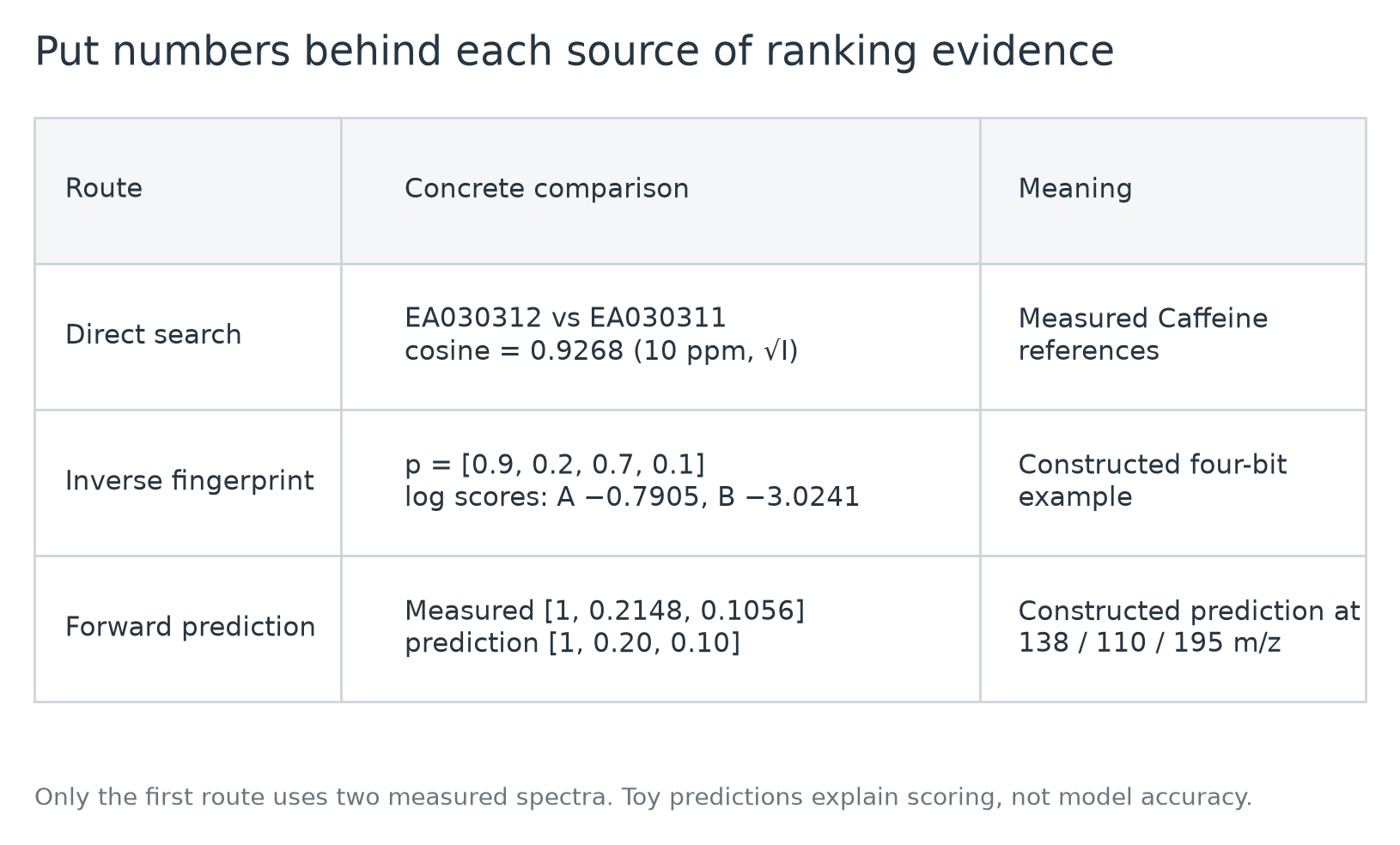
What does each approach contribute, and where can it fail? Comparing the three directions with analog propagation and generation clarifies what each experiment is testing.

Approach	Evidence or candidates added	Failure to examine	Results to record first
Direct spectral search	Agreement with an actual reference measurement	No correct reference, or a large condition mismatch	Rank and peak agreement, separated by reference availability
Analog propagation	Candidates supported by related reference structures	Spectral similarity does not imply structural similarity	Candidate Recall@K and structural relationships among errors
Fingerprint prediction	Substructures suggested by the observation	Isomers share similar fingerprint features	Ranking among same-formula candidates
Forward prediction	How well a candidate explains the observed spectrum	Unsupported conditions or inaccurate fragments and intensities	Per-molecule rank changes and added runtime
De novo generation	Structures outside a fixed database	Valid SMILES do not guarantee the correct structure	Exact-key generation rate and damage to existing correct ranks

This table provides comparison criteria. It is not a measured performance or runtime ranking of particular models.

Expensive calculations need not run on every candidate

Predicting spectra for hundreds of thousands of structures can be costly. Fast retrieval and fingerprint scores can first reduce the pool, with more detailed computation reserved for the top K.

As a design example, 400 molecules with 100 candidates and 3 observation conditions each would require up to 120,000 candidate–condition comparisons. This is not an exact workload forecast for the hidden test. The actual number depends on spectra per molecule and whether repeated candidate–condition computations can be cached.

Evaluate added runtime and memory alongside MRR. A method that exceeds the execution limit cannot be used unchanged in the submission, even if it is accurate.

Separate measured evidence from a hypothetical model output

Use the 75% Caffeine observation at [138.0662, 110.0713, 195.0878]: its normalized intensities are [1.0000, 0.21480, 0.10565]. Suppose a candidate-conditioned model predicts [1.0, 0.20, 0.10] at those masses and a competing prediction gives [1.0, 0.02, 0.50]. Both explain the base peak, but the second underpredicts the 110 fragment and overpredicts precursor survival. These invented predictions explain what rescoring compares; neither was generated by an actual checkpoint. A real score must also include missing/spurious peaks beyond this three-peak excerpt.

Before testing a downloaded forward model, make its input contract explicit: supported adducts, whether it consumes eV or normalized energy, instrument conditioning, mass range, output bins, and training structures. A checkpoint trained for [M+H]+ cannot automatically validate negative-mode rescoring. Likewise, a formula-conditioned method cannot be fed the test molecule’s unknown formula without adding a formula-estimation stage.

These routes still evaluate structures already proposed. If no database contains the answer, the system also needs a way to propose a new structure that explains the observations.

10. Molecules outside the database: the role of de novo generation

For Class 3, PubChem and COCONUT do not supply the correct structure. When our candidate pool lacks it, we need a route that can propose structures beyond that pool. De novo structure generation can generate SMILES from spectra, search molecular graphs under a formula constraint, or modify existing candidates.

MassSpecGym treats retrieval, de novo generation, and spectrum simulation as separate tasks. FOAM illustrates formula-constrained structure search with a spectrum predictor used to evaluate candidates.

A generated candidate must pass several different checks:

1. Can it be parsed? Does RDKit accept the SMILES?
2. Do its mass and formula fit? Is it consistent with precursor information?
3. Is it chemically plausible? Does it avoid inappropriate structures or bonding?
4. Does it explain the spectrum? Does the fragment evidence support it?
5. Is its connectivity correct? Does its scoring key match the target?

A high success rate at the first step can coexist with a low success rate at the last. A structure with a very similar fingerprint still earns no credit if its scoring key is wrong.

Deciding where a generated candidate belongs

Automatically inserting a generated structure at rank 1 can displace a correct answer. If a false candidate moves a correct rank-1 answer to rank 2, that molecule’s contribution falls from 1 to 0.5.

Appending candidates to unused slots while preserving the original order leaves earlier correct ranks unchanged. Exceeding 25 candidates or inserting a candidate in the middle has different consequences. A generation method therefore needs validation of both candidate quality and whether its candidates deserve to displace existing ones.

Before training a large generator, I want to determine whether candidate omissions or ranking errors dominate. If many answers already enter the pool but lose to incorrect same-formula structures, improving ranking is a more direct next experiment.

Combining retrieval, prediction, and generation creates more ways to obtain a strong local score. We still need to distinguish learning to interpret new molecules from having already seen their answers. The next section defines a comparison that can separate those explanations.

A concrete graph-edit example and its limit

Take Isoeugenol, COc1cc(C=CC)ccc1O. Moving the side-chain double bond gives Eugenol, COc1cc(CC=C)ccc1O, without changing C10H12O2, exact mass, or DBE = 5. Both strings are valid, but their metric keys differ. This is a concrete example of proposing a missing candidate through graph editing; it does not establish which structure a measured spectrum supports. Withholding Eugenol from a known-structure benchmark creates a generation surrogate, not a newly discovered molecule.

For formula-constrained search, evaluate the formula shortlist first. If it contains the correct formula for 90 of 100 queries, then at most those 90 can be recovered by a search strictly restricted to the shortlist. Graph validity, unique metric-key yield, exact-key recall, rank after fusion, and model-call count should be recorded separately. Increasing a beam from 100 to 1,000 strings can mostly add duplicates, so unique structures and exact recovery matter more than string count.

11. Structure-level OOF: what must be out of fold?

Out-of-fold (OOF) predictions are generated for examples excluded from the corresponding model’s training fold. They let us compare models and learn ensemble weights on predictions made without fitting those targets. OOF is a prediction protocol, not an ensemble architecture. Averaging several seeds trained on the same structures does not create OOF predictions. Grouped cross-validation · Stacking

One split must follow a molecule through the entire system

Use the metric’s normalized structure key as the group. All Caffeine spectra in our measured example belong to RYYVLZVUVIJVGH, so they enter the same outer fold even if their collision energies or source libraries differ. The same applies to a different SMILES or tautomer that canonicalizes to that key. A random row split would let a model train on one Caffeine spectrum and validate on another.

Figure 11. Apply one structure-key exclusion across all references and supervised stages. The query measurements remain prediction inputs, while the graph remains a candidate for Class 2. This is a split design using known records, not a completed validation result.

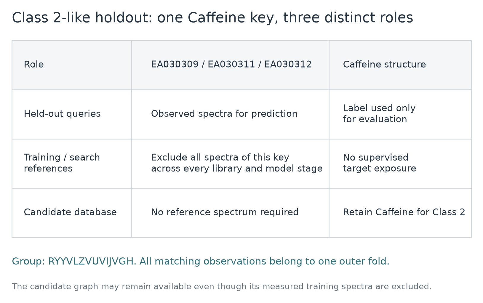
For a Class 2-like comparison, the held-out molecule has three distinct roles. Its query spectra are available for prediction; its reference spectra and supervised training targets are unavailable; its structure remains a permissible candidate. Treating all three as one table and deleting the molecule everywhere silently changes the experiment into candidate exclusion.

Component	Treatment of an outer-held-out Caffeine structure	Reason
Reference spectral libraries	Remove every matching normalized key across libraries.	Prevent direct recovery from a withheld structure’s reference spectrum.
Fingerprint encoder and spectrum predictor	Exclude its supervised examples during fitting; audit fixed pretrained checkpoints separately.	A retrieval exclusion cannot undo memorization in model weights.
Structure candidate database	Retain Caffeine for Class 2; remove it for a Class 3-like generation test.	Candidate availability defines the task.
Ranker rows, calibration, ensemble weights, stopping thresholds	Fit without the outer fold.	Their labels and decisions are part of the learned pipeline.
Masses and fingerprints computed from candidate structures	May include Caffeine as candidate-side information for Class 2.	A deterministic candidate descriptor is not an observed target spectrum.

Base-model OOF is not an independent score for the stacker

For molecule \(u\) in fold \(f(u)\) and candidate \(c\), let the OOF output of model family \(m\) be

\[z_{u,c}^{(m)}=s_m^{(-f(u))}(\mathcal S_u,c).\]

The superscript means that fitting excluded that fold. Store a candidate table indexed by molecule key and candidate key. Candidate A in one model’s row 0 must not accidentally align with candidate B in another model’s row 0. For models with different pools, explicitly form the union and encode a missing candidate; a rank-based score can assign zero support to an unreturned candidate rather than treating it as rank 1.

Suppose 5 folds contain 1,000 structures each. A fingerprint model makes OOF predictions for all 5,000. If a ranker then fits all 5,000 OOF candidate tables and we report its score on those same tables, the ranker has seen the evaluation labels. The encoder predictions were OOF; the complete pipeline was not.

A strict design uses an outer structure split to estimate the whole pipeline. Inside the outer training structures, generate inner-OOF encoder features to fit the ranker and any calibration. Refit the encoder on the outer training structures, run it on the outer held-out queries, and score those queries with the ranker that never saw their labels. Repeat for each outer fold. If ensemble weights are chosen from these outer predictions, reserve another untouched evaluation panel—or use another outer selection layer—to estimate the selected ensemble without tuning on its own reported result. The extra fitting cost is real; a smaller fixed development/selection/audit split can be a practical alternative.

Splitting a globally generated encoder-OOF table again for ranker CV is not automatically independent: encoders that produced ranker-training rows may have used the outer evaluation structures. Regenerate those features entirely within the outer training set. If calibration or a routing gate is learned from ranker scores, distinguish cross-fitted ranker outputs from encoder OOF features. An outer set preserved throughout still provides an independent evaluation of the complete procedure.

Candidate generation must also be fold-correct. Measure retrieval as it actually runs. Injecting the known answer into each validation pool produces a useful conditional ranking diagnostic, but not an end-to-end MRR estimate.

A numerical ensemble example

Consider three held-out molecules. In this constructed example, model A ranks the true candidates at [1, 2, 25], model B at [2, 1, 25], and a candidate-aligned blend at [1, 1, 25]. Their MRR values are 0.5133, 0.5133, and 0.6800. The blend result is an assumed outcome for the example, not something that can be deduced from true-answer ranks alone: actual fusion requires the scores or ranks of all competing candidates.

By contrast, a third model that returns exactly A’s order adds no ranking information even if its standalone score is equally strong. On real OOF predictions, inspect both candidate-score dependence and per-molecule reciprocal-rank changes. Bootstrap molecules, not their repeated spectra. Report candidate Recall@K, MRR, Top-1, and subgroup results by adduct, mass, instrument/source, and number of observations. A scaffold holdout is a further stress test for chemical extrapolation, not a substitute for specifying the original task.

A public pretrained checkpoint with unknown training membership remains an important limitation. Calling the downstream split GroupKFold does not make the upstream representation independent. Record that result as evaluation with a fixed public model unless its relevant training exclusion is established.

12. Where does the public work stand now?

The public starting point has progressed well beyond an isolated nearest-spectrum search. Several reusable components now fit together: a library of measured spectra, structure candidates from training data and COCONUT, predictors of structural fingerprints, and learned models that combine the resulting evidence. The question for a newcomer is which part to reproduce first and which remaining error to investigate.

Read the leaderboard as a dated measurement

The public leaderboard archive downloaded on September 27, 2026, at 02:59:30 UTC contained 1,608 scored team entries. The table below summarizes that archive; it is not a live counter. Public leaderboard

Observation in that snapshot	Value	How to interpret it
Highest public MRR@25	0.425	A reference for the public frontier; the number alone does not reveal the method.
Second and third public scores	0.421 / 0.412	Several teams were above 0.40.
Median team score	0.292	Half the downloaded team entries were at or below this value.
Teams scoring from 0.335 through 0.342, inclusive	263	Many entries occupy a narrow band near the public baselines. This count does not prove they use the same code.

An MRR of 0.425 does not mean that 42.5% of molecules were identified at rank 1. It averages reciprocal ranks, so different combinations of first-place answers, lower-ranked answers, and misses can produce it. Nor does the public ranking tell us how the private ranking will turn out. For a small public-score difference, the useful follow-up is to ask which molecules changed in a held-out comparison, not to infer a new scientific capability from the decimal alone.

What the public notebooks actually add

The notebook score panels below were checked during the same September 27 review. Scores are tied to the versions indicated; they are not a controlled comparison in which only one component changed. In particular, a notebook’s Best Score may belong to an older version than the source currently displayed.

Public notebook and checked version	Displayed public score	Contribution to the story
Analog Propagation, best-scoring V10	0.335	A shared foundation: retrieve measured spectra, extend evidence through related structures, and combine it with learned features. The page displayed V32 at review time; 0.335 belongs to V10.
Fast Spectral Cosine baseline, V17	0.339	Shows how processing choices and an inherited multi-channel pipeline develop beyond the simple-search name.
Two Rankers, One Engine, V1	0.337	Makes alternative rankings and their combination explicit within a common candidate engine.
Evgen Dvorkin’s Enveda CASMI notebook, V15	0.342	A public two-ranker variant that provides a practical reproducible starting point.
Ahmed Beratozer’s v3 inference, V6	0.358	Adds a separately controlled PubChem candidate route to a richer engine. Some required inputs are private.
Ahmed Beratozer’s v4f inference, V1	0.362	Includes richer ranking evidence and ICEBERG rescoring. Private inputs limit independent reproduction from the notebook alone.

These examples suggest a progression: recognize what is already measured → extend to known structures without reference spectra → distinguish increasingly similar candidates. They do not establish a causal gain for every added component. A higher-scoring notebook can change its training data, candidate set, features, and model together. The 0.362 result, for example, is evidence about that submitted pipeline, not a measured “ICEBERG improvement” by itself.

The public code also makes clear why a model name is an incomplete recipe. In a notebook’s Input tab, structure collections supply possible answers; fingerprint weights turn spectra into structural evidence; simulated ranking rows teach the order of candidates; package files make offline execution possible. Reproducing the combination requires compatible versions of those inputs. Reading code that depends on private weights can still teach an idea, but it does not supply a runnable baseline.

What seems to be holding progress back?

A participant’s account of roughly 30 submissions describes frequent cases where the correct structure is available but a same-formula candidate wins instead. The discussion of score plateaus also reports examples where extra features or models produced little improvement. These are participant observations under their own experimental conditions, not a measurement of the entire hidden set.

Our eugenol/isoeugenol example shows the kind of decision involved. A mass filter can admit both; broad structural features may support both; the useful additional signal is something that changes their relative order for the right reason. A larger database can rescue a missing answer, but if it mostly adds close distractors, the ranker faces a harder task. Better candidate coverage and better ordering must be measured separately.

This is why I would treat the public 0.34 region as a working baseline to understand, rather than a score to imitate through repeated parameter changes. The leading public scores leave room above it. They do not tell us whether that room comes from candidate coverage, ranking, generation, or a combination that leading teams have not disclosed.

Where this project is, and what remains unproven

In this project, a submission based on the public two-ranker engine has completed with public MRR@25 = 0.342. That is a reproduced baseline, not a newly demonstrated modeling improvement. This value was checked against the project submission record and Kaggle’s completed-submission response.

The next unresolved task is a trustworthy local comparison, especially for Class 2: remove a held-out structure’s reference spectra and supervised training exposure while retaining the structure in the candidate pool. The project has not yet established an independently validated gain from a new forward-model, ranking, or generation method. This distinction places us at a useful starting point: the system runs and has a hidden-evaluation reference score; now we need evidence that can tell us which change deserves to become the next version.

Read resources in the order of the decision they support

Resource	Inspect first	Question for this project
Fast Spectral Cosine baseline	Its library-search component: peak processing and mass indexing	How is direct retrieval implemented? The full notebook score includes other channels.
Analog Propagation baseline	Candidate pools, analog support, and fingerprint scores	How are unmeasured structures scored?
Two Rankers, One Engine	Score fusion and molecule-level outputs	How does each source of evidence affect the final order?
MassSpecGym	Retrieval, de novo, and simulation tasks and splits	How are the different abilities evaluated separately?
MIST · DreaMS	Spectral representations and structural-feature prediction	Can learning add information missing from retrieval?
ICEBERG/GLACIER	Candidate spectrum prediction and condition inputs	Can same-formula candidates be distinguished more reliably?
FOAM	Formula-constrained search and model-call budgets	Can useful new structures be proposed within limited computation?

13. Train efficiently, then choose an ensemble that fits the submission budget

CASMI has the familiar Kaggle problem of selecting complementary models from held-out predictions, with an additional complication: different models can propose different candidate sets and share expensive intermediate computations. The objective is the MRR of the final candidate order under a runtime and memory budget, not the sum of standalone model scores.

Three different clocks

Budget	What it includes	Practical consequence
Offline development	Model training, fold predictions, candidate construction, ranker training, and ensemble selection	A 9-hour inference limit is not a universal 9-hour limit on all prior training.
Kaggle development GPU allocation	Account usage during development and version runs	Official guidance describes 30 hours per week, sometimes more depending on demand and resources. Check the actual allocation.
One submitted notebook	Loading, preprocessing, search, any runtime fitting, inference, fusion, and CSV validation	Both CPU and GPU submissions must finish within 9 hours, with internet disabled.

These are separate constraints. The organizers have explicitly allowed training in a private external cloud environment and bringing the weights back to Kaggle. This does not permit publishing restricted competition data. Code requirements · Kaggle GPU allocation · Host clarification

As a budget calculation, three model families × five folds × two seeds × two GPU-hours per fit already require 60 GPU-hours, before OOF feature generation or a final refit. Assuming each fit consumes two hours of the selected backend’s quota, under a 30-hour weekly allocation, that equals two full weekly allocations. Parallel GPUs reduce elapsed time but do not remove accelerator-hour cost. This is why validating a new representation on a fixed development panel before expanding to every fold and seed can matter more than shaving seconds off a CSV write.

What the reproduced engine actually ensembles

The current public-derived engine loads two FPNet views: a spectrum-level model and a merged-spectrum model. It also fits 16 pointwise gradient-boosting classifiers on one ranking table and 12 on another, varying seeds and class priors. Their inputs contain 31 and 51 features respectively. Each group averages probabilities, then the two groups contribute mostly through a 0.88/0.12 blend of within-molecule normalized ranks. This is not a blend of raw probabilities, and the shared-row seed ensembles do not establish whole-pipeline OOF validation. Public engine lineage

Those 28 small classifier fits currently occur during notebook execution, so their cost belongs to the submission budget. Serializing fitted classifiers beforehand could move that cost offline, but the exact data, versions, numerical behavior, and output equivalence would need checking. It is an optimization proposal, not a change already validated in this project.

Measure mixed CPU/GPU work before choosing a remedy

Existing project logs provide a concrete scale. Both runs below processed the visible 1,213-spectrum / 400-molecule input. They are execution measurements, not hidden-set accuracy or runtime guarantees.

Figure 12. Existing notebook logs on 1,213 spectra and 400 molecules. Intervals combine multiple operations; in particular, MetFrag and GBM fitting are not timed separately. The setup segment is the rounded total less the reported intervals. These are visible-input measurements, not hidden-test forecasts.

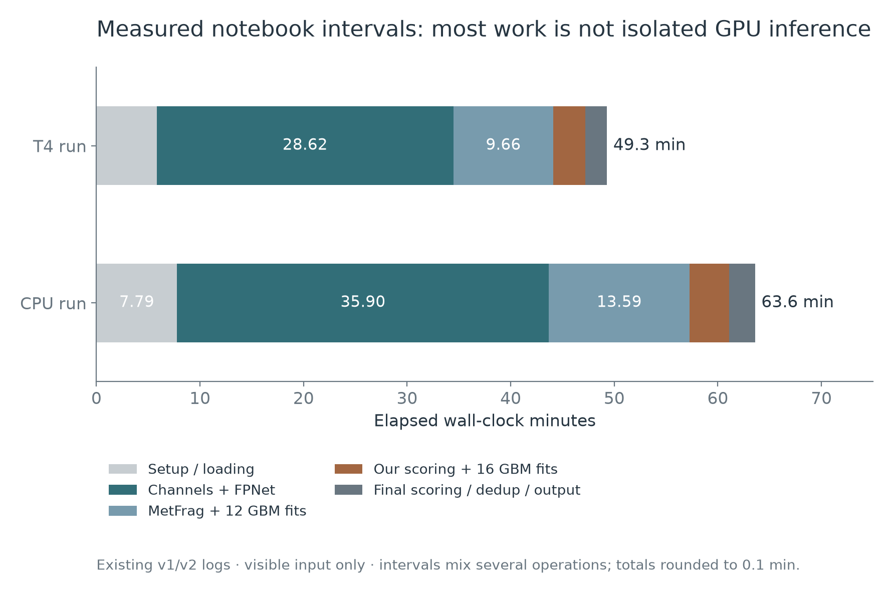
Logged interval	T4 run, minutes	CPU run, minutes	What is actually included
Test loaded → MetFrag begins	28.62	35.90	Spectral channels and FPNet; not isolated GPU inference.
MetFrag begins → 12 GBM fits complete	9.66	13.59	Fragment features and fitting 12 GBMs.
12 GBM fits complete → 16 GBM fits complete	3.08	3.83	Scoring in that route and fitting 16 GBMs.
16 GBM fits complete → submissions ready	2.10	2.49	Remaining scoring, deduplication, and submission-table construction.
Reported elapsed time through CSV construction	49.3	63.6	Manifest elapsed time; excludes later manifest hashing/platform finalization.

A faster accelerator cannot eliminate CPU-side search, loading, or ranker fitting. Nor should we multiply the entire visible time by a spectrum-count ratio: setup is mostly fixed, spectral inference grows with observations, and candidate scoring grows with the number and density of candidates. The logs motivate finer profiling; they do not isolate the causal speedup of one component.

Where training compute is best spent

Start with structurally different model families that might correct different mistakes: a spectral encoder, a forward predictor, and a ranker using independent evidence. First compare one controlled configuration of each under the same group split and data budget. For expensive training, use a smaller fixed screening panel, then promote only useful configurations to full folds and multiple seeds. Screening scores are selection evidence; retain an untouched audit set for the chosen system.

Store candidate-aligned OOF predictions once for each fixed model, fold, and candidate policy. Weight searches and light ranker comparisons should reuse these outputs rather than retrain the encoder. Shared raw parsing and deterministic candidate descriptors can also be reused. Learned transformations, target-derived reference libraries, and supervised features must respect the fold boundary; caching them globally does not make them safe to share.

Select epochs and early stopping without the outer evaluation labels. Compare improvements at a stated compute budget, including failed or discarded fits. If two extra seeds reproduce the same molecular errors while a new representation resolves them, the latter can be a better use of the next training allocation. The evidence is paired rank improvement, not architectural novelty.

OOF training does not require deploying every fold model

Five-fold training leaves five checkpoints. At submission time, one can use all five, a validated subset, or one model refitted on all permitted training data. These choices trade inference cost against variance and training-set size. A full-data refit can also change score calibration. A ranker trained on one-fold OOF features may receive a different feature distribution from a five-model average; evaluate the deployment recipe, not only the existence of five checkpoints.

Averaging all five global fold models on a validation molecule is not OOF: four may have trained on it. To evaluate the deployed ensemble, every contributing model must exclude the outer-held-out molecule.

For illustration, with 400 molecules, three spectra each, and five fold replicas of each view, a single-spectrum plus merged-spectrum encoder uses approximately 5 × (1,200 + 400) = 8,000 sequence evaluations. A forward model applied to 100 candidates at all three conditions needs up to 5 × 400 × 100 × 3 = 600,000 candidate–condition evaluations. The operations differ in size, so their count ratio is not a speed ratio. If a measured, batch-amortized forward cost were 10 ms each, that forward stage alone would take 100 minutes. The 10 ms is an illustrative assumption, not a measurement here.

Model selection is a constrained portfolio problem

For a serial execution schedule, write the cost as

\[\begin{aligned} T(\mathcal M,g)&=T_{\mathrm{load}}+T_{\mathrm{shared}}\\ &\quad+\sum_{m\in\mathcal M}T_m^{\mathrm{incremental}}(g)\\ &\quad+T_{\mathrm{runtime\ fit}}+T_{\mathrm{output}}. \end{aligned}\]

Shared candidate indices or encoder features count once. Incremental cost depends on which other models are already present and on the routing rule \(g\). With parallel execution, measure the actual dependency path and contention instead of assuming the serial sum predicts wall time.

The selection problem is then

\[\begin{aligned} \max_{\mathcal M,w,g}\quad &\widehat{\operatorname{MRR}}_{\mathrm{selection}} \!\left(\operatorname{Fuse}_{w,g}(\mathcal M)\right)\\ \text{subject to}\quad &\widehat T_{\mathrm{stress}}(\mathcal M,g)+\Delta\leq9\ \mathrm{h},\\ &M_{\mathrm{peak}}\leq M_{\mathrm{available}}. \end{aligned}\]

Here \(w\) denotes fusion parameters, \(\Delta\) a measured operational reserve, and the hat indicates an estimate. This does not guarantee performance on unseen workloads; explicit workload limits and complete-run tests are still needed. The selected system’s final accuracy is assessed on the untouched audit split from Section 11.

Consider this constructed example, where shared work costs 0.75 hours and incremental model costs are A = 2.0, B = 1.5, C = 4.5 hours. The MRR entries represent hypothetical results after actually fusing complete candidate lists; they are not averages of model scores.

Selected models	Hypothetical selection MRR	Total hours, including shared work	Fits an illustrative 8-hour working budget?
A	0.340	2.75	Yes
B	0.330	2.25	Yes
C	0.350	5.25	Yes
A + B	0.360	4.25	Yes
A + C	0.365	7.25	Yes
A + B + C	0.367	8.75	No

With a chosen one-hour reserve, A + C wins among these options even though all three have the highest estimated MRR. The reserve is a design assumption, not a Kaggle rule. A + B is cheaper and could be preferable if workload uncertainty is larger. The ratio of incremental MRR to incremental time is a useful screening statistic, but interactions make greedy selection unreliable as a global optimizer.

Reduce computation where the model actually spends it

For a fingerprint model, encode each observation once, then score candidate bit vectors against its logits. For a forward model, cache by structure, supported condition, and model version, then batch candidate inference. Reusing an unsupported energy or adduct silently changes the prediction problem. A candidate cap K = 100 can remove the answer that ranked 101st in the cheap stage; measure Recall@K before adopting that cap.

Storage format matters too. A 711,705 × 6,930 binary fingerprint matrix occupies about 0.574 GiB bit-packed, 4.59 GiB as uint8, or 18.37 GiB as float32, excluding overhead. Unpacking every candidate at once defeats the memory saving; scoring blocks should bound the working set. CPU thread oversubscription, repeated weight loading, and tiny GPU batches are separate profiling targets.

A selective forward-model gate can use quantities available at inference—such as disagreement between rankers or a narrow score margin. It cannot use “the true answer currently ranks second.” Fix and validate the gate using held-out predictions, including errors on confidently wrong molecules. Stress-test large candidate pools, long peak lists, and molecules with many observations, and record peak RAM/VRAM and total wall time.

A practical execution design first prepares a valid baseline for every molecule, then performs bounded expensive reranking. Candidate limits, beam limits, stopping rules, and fallback behavior are part of the evaluated model policy. A timeout workaround that changes which molecules receive which model can change accuracy; it is not merely an implementation detail.

External resources and reproducibility

A code license does not establish the license or training provenance of linked weights. Check the exact checkpoint. The organizers’ pretrained-model clarification distinguishes eligible resources from models derived from restricted data. An earlier CFM-ID permission does not answer the later CFM-ID 4/METLIN provenance question, which remained unanswered at this article’s check.

Competition data have CC BY-NC terms and sharing restrictions. The public experimental spectra reproduced here come instead from the three Eawag/MassBank CC BY records, with their authors, original files, and transformations retained in the figure provenance. Only source-level aggregate counts are shown from competition training data. Rules · Organizer announcement

14. How should the first experiment begin?

For a newcomer, a small search example and a competitive public-engine reproduction serve different purposes. Use the first to understand inputs and scoring, then use the public two-ranker from Section 12 as an identifiable comparison baseline. This project has already submitted that baseline; its next milestone is independent validation and failure analysis.

Step 1: check inputs and the answer definition

There is no need to load the entire training set into memory at the start. Parquet is column-oriented, so we can inspect its schema and a small batch. This example assumes the local project has data/train.parquet; in Kaggle, substitute the actual path of the attached input.

from pathlib import Path
import pyarrow.parquet as pq

path = Path("data/train.parquet")
pf = pq.ParquetFile(path)
print("rows:", pf.metadata.num_rows)
print("columns:", pf.schema_arrow.names)

columns = ["normalized_smiles", "precursor_mz", "adduct",
           "ms2_mzs", "ms2_normalized_intensities"]
batch = next(pf.iter_batches(batch_size=8, columns=columns))
sample = batch.to_pydict()
for mzs, intensities in zip(sample["ms2_mzs"],
                           sample["ms2_normalized_intensities"]):
    assert len(mzs) == len(intensities)
    print("peaks:", len(mzs), "base peak:", max(intensities))

Check column names, array lengths, missing values, and normalization ranges. This also makes the distinction visible: training data contain structures, while test structures must be predicted. Then check the scoring-key behavior from Section 2.

Alongside the environment setup, check the training-data correction notice: some samples gained water-loss adducts. It is a concrete example of a data update that can affect neutral-mass conversion and candidate filtering.

Step 2: fix the validation molecules and candidate pool

Save the evaluation molecule list and split definition first. For a Class 2-like panel, remove target spectra across all libraries while retaining the structures as candidates. Start with a small panel relevant to natural products and timsTOF, then check a broader set of structures to avoid optimizing only that panel.

Measure candidate Recall@K next. If correct answers are absent, investigate mass tolerances, adduct handling, database coverage, and normalization before changing the ranker.

Step 3: establish retrieval and ranking baselines

Run a baseline combining direct search, analog support, and fingerprint scores. Remove one score at a time to see what contributes. Keep candidates and validation molecules fixed so that the differences are interpretable.

The output should include per-molecule correct ranks and leading incorrect candidates, alongside mean MRR. Inspecting molecules whose answer ranks second can provide a concrete reason to improve ranking features.

Step 4: add one hypothesis

One experiment I am considering is adding forward-model scores for difficult same-formula candidates. Compare the existing ranking with a ranking that adds forward features to the same candidates. Changing the pool and the observation spectra at the same time would obscure the cause of any improvement.

Observed failure	Change to test next	Measure alongside it
The answer is absent from the pool	Candidate databases, mass windows, and adduct handling	Recall@K and candidate counts
The answer is present but loses to same-formula errors	Forward scores and ranker training with difficult negatives	Per-molecule rank changes and runtime
Performance drops sharply with few observations	Condition-aware score aggregation and training sampling	Performance with one, a few, and all observations
A particular ionization condition performs poorly	Condition-specific processing and model support	Candidate omissions and ranking errors under that condition
The correct structure cannot be included in the retrieval pool	Bounded de novo search	Exact-key generation rate and harm to existing candidates

Consider a hidden-test submission after the change helps validation and fits the runtime limit. Successfully running the public placeholder only establishes the format-checking part of this process.

The approach I would prioritize now

My working choice is a retrieval-centered system with learned ranking and selective spectrum prediction. It gives each method a concrete job: direct matches handle familiar molecules; analog and fingerprint evidence extend the search to known but unmeasured structures; a forward model is tested where similar candidates remain hard to separate. Structure generation stays a separate branch for cases the fixed databases cannot cover.

That choice follows the public evidence in Section 12, but it still needs validation on our own molecules. I would first preserve the reproduced public engine as a control, establish a trustworthy Class 2-like holdout, and inspect its leading errors. If same-formula ranking errors dominate, the next comparison is a forward-model feature on the same candidate pool. If missing candidates dominate instead, database coverage and candidate construction take priority. The experiment decides which part deserves more effort.

The first changes should also be small enough to interpret. Adding a larger pool, a new fingerprint model, a new ranker, and generation at once can move the score while leaving us unable to explain why. A useful improvement should identify the molecules it recovers, the molecules it harms, and the additional runtime it needs.

A first week organized around answers

The following is a proposed sequence of milestones, not a promise that training or data preparation fits a fixed number of days.

Milestone	A concrete result to keep	Question answered
Read one molecule end to end	Its conditions, spectra, candidate structures, normalized keys, and final row.	Do we understand what the pipeline is predicting?
Run the unchanged public baseline	A pinned notebook/input version and an execution record.	Can we reproduce the procedure?
Build the held-out comparison	Frozen molecule IDs, separate spectral and structure pools, baseline per-molecule ranks.	Is our local score testing the intended kind of unknown?
Inspect the failures	Candidate misses, same-formula errors, and condition-specific regressions.	Which stage should change first?
Test one change	Paired rank changes, MRR, candidate recall, and total runtime.	Is the new evidence useful enough to keep?

Make the next comparison reproducible at the candidate level

For the first forward-model comparison, freeze the query groups, reference exclusions, baseline candidate pool, and base scores. Save rows such as (outer_fold, molecule_key, candidate_key, baseline_score, forward_score, is_correct), plus model/data hashes and condition support. Ground truth belongs in the evaluation table, never in inference-time routing. Preserve a sufficiently deep candidate list, not only the final 25, so fusion can promote candidates that individual models ranked lower.

Generate fold-correct features, fit fusion on development/inner-OOF data, select its configuration on the selection panel, and assess the chosen pipeline on the untouched audit panel. Report per-molecule ΔRR and aggregate ΔMRR, coverage changes, total and incremental runtime, and peak memory. If the forward route recovers ten rank-2 answers but demotes ten rank-1 answers to second, its net change is zero before considering any other molecules. Counting recovered cases alone would hide the failure.

This produces an OOF prediction bank for inexpensive combination searches and a measured deployment comparison. It gives a concrete decision: retain the new route, restrict it with a validated gate, or reject it and spend the next training budget elsewhere.

15. How I expect the competition to develop

The public work already contains more than a simple spectral lookup: candidate expansion, learned structural features, and multiple ranking signals are available. My expectation is that the next useful gains will depend increasingly on which uncertainty a method resolves. The following are possible developments, not reports of undisclosed leading architectures.

First, shared baselines make small variations less informative

When many notebooks inherit the same candidate pool, fingerprint weights, and ranking features, changing seeds or blend weights can reshuffle a few close decisions without introducing new chemical evidence. Such changes can still help, but a small public-score gain alone does not tell us whether the improvement will persist on the private split.

I expect stronger comparisons to ask which held-out molecules improve across several observation-count and source conditions. If a gain disappears when the reference library or validation source changes, the next problem is transfer. If it persists across those comparisons, it becomes a more credible candidate for final selection. This is why keeping the baseline identifiable matters as the notebooks evolve.

Next, distinguishing close structures becomes more valuable

If the correct answer is already in a manageable candidate pool, the opportunity is to separate it from chemically plausible alternatives. A hard negative is an incorrect candidate that is difficult to distinguish—for example, a molecule with the right mass and formula but different bond connectivity. Training against those alternatives asks a more relevant question than separating the answer from arbitrary unrelated molecules.

Condition-aware spectrum prediction, better use of neutral losses, and fingerprint models trained without evaluation-structure overlap could provide additional evidence. They could also repeat information the ranker already has. The evidence for this direction would be consistent improvements in the ranks of same-formula candidates, with acceptable costs and without undoing reliable reference matches. The participant reports in Section 12 make this worth testing; they do not establish that adding a named forward model is sufficient.

Generation becomes useful when it supplies answers the rest cannot reach

The absence of Class 3 answers from PubChem and COCONUT gives structure generation a clear role: propose answers that a pool built from those databases cannot supply. Its competitive value depends on generating the exact accepted structure, recognizing when that generated candidate deserves a high rank, and completing the search within the inference budget. A chemically valid string alone achieves none of those three goals.

I would expect generation to be tested first with a limited search budget and an explicit comparison of recovered answers against displaced good candidates. If Class 3-like validation shows useful exact-key recovery and reliable ranking, it deserves a larger share of computation. If it mostly produces plausible but incorrect structures, better retrieval and ranking remain the more productive investment for the cases they can solve. We do not know the hidden class mixture well enough to turn that trade-off into a fixed allocation in advance.

What could change this plan?

A new well-documented candidate resource could change coverage. A permitted checkpoint with useful measurement-condition support could change the cost of spectrum prediction. Data corrections or organizer rulings could change which inputs should be used. The training-data update and the checkpoint-specific CFM-ID question are examples of developments that deserve a targeted recheck. Training update · Model clarification · Open CFM-ID question

Each such event should lead to a specific comparison while preserving the previous control. My present bet is on a system that knows when a library match is strong, distinguishes close candidates better, and spends expensive computation on the unresolved cases. I would revise that bet if the held-out evidence showed that candidate coverage or generation, rather than ordering, accounted for most recoverable errors.

The likely bottleneck is evidence per unit of compute

A plausible next phase is competition between candidate-aligned OOF ensembles, not simply the largest collection of checkpoints. A new encoder needs to show marginal benefit over existing representations; a forward predictor needs to resolve isomers after paying its candidate-by-condition cost; a generator needs to add accepted keys that fixed pools miss. For example, a route adding 0.002 MRR at four extra hours is a different deployment proposition from one adding 0.010 at twenty minutes. Those are hypothetical comparisons; only controlled measurements can place real methods on that curve.

I would track the best independently checked MRR for each feasible runtime range, alongside candidate coverage and subgroup failures. A useful permitted checkpoint, a cheaper distillation, or a validated gate can change that frontier. Repeated leaderboard-only tuning cannot tell us whether the frontier moved or a small public subset was fitted more closely.

16. Dates and the first milestone

The official deadlines are all at 23:59 UTC, which is the following morning in Korea. Competition timeline

Event	UTC	Korea Standard Time
Entry and team-merger deadline	December 7, 2026, 23:59	December 8, 08:59
Final submission deadline	December 14, 2026, 23:59	December 15, 08:59

At the verification date, the rules allow 5 submissions per day, 2 final selections, and teams of up to 5 members. Total prizes are $50,000. Recheck the rules and schedule announcements before entering or making final selections.

The first experiment should show which molecules retrieval solves, which suffer ranking errors, and which lack the correct candidate altogether. That distinction gives us a reason to choose the next model. CASMI offers a way to learn how to connect incomplete measurements with limited chemical knowledge and propose structural candidates that can be tested.

---

References and what was checked

The structure and mass calculations, scoring-key examples, and illustrative MRR calculation were checked with RDKit 2026.03.3. Isotope-mass sums, adduct and neutral-loss differences, DBE, and center-of-mass energy examples were also checked numerically. The Parquet example was checked on a small batch from the local training file.

The Caffeine figures reproduce Eawag/MassBank records EA030309, EA030311 and EA030312 by Stravs M, Schymanski E and Singer H (Department of Environmental Chemistry, Eawag; Copyright 2012 Eawag), each labeled CC BY in its source record, without a license version specified. Peak intensities were divided by the original base-peak signal; nominal collision-energy percentages were not converted to eV. Original files, source commit and hashes, transformations, and the plotting code are retained with the figure provenance. The kinetics, candidate orders, four-bit predictions, forward outputs, and ensemble portfolio are labeled calculated or constructed examples. The runtime chart uses existing project logs. All 12 body figures are shared with the Korean edition. 30% source · 60% source · 75% source

The leaderboard distribution was calculated from the full public ranking downloaded on September 27, 2026, at 02:59:30 UTC. Six notebook scores and their version links were checked in the actual score panels that day. Team best scores were not substituted for notebook results; the comparison is not a component-level ablation. The project’s 0.342 comes from a baseline submission completed before this editorial revision.

Descriptions of public research models are based on their authors’ code and documentation. No model training or Kaggle submission was performed for this article. Illustrative scores are labeled separately from aggregate dataset statistics.

Further reading, grouped by purpose:

• Competition reference: Overview, evaluation, and timeline, input data, official metric, and rules.
• Physical-chemistry foundations: NIST isotope masses, LC/MS and ionization, CID definition, mass resolving power, and formula constraints and their limitations.
• Fragmentation in more depth: Protonation and small-molecule CID prediction, MassKinetics on energy transfer, kinetics, and observation, and an application of RRKM.
• Understanding the data: Enveda-180 processing code, COCONUT, PubChem, and MassSpecGym.
• Retrieval and structural features: Analog Propagation, Spectral Cosine, matchms, MIST, and DreaMS.
• Detailed ranking and generation: ICEBERG/GLACIER and FOAM.
• Validation and practical discussions: Structural duplication in natural-product CV, plateaus across variants, ranking lessons from submissions, and conditions for pretrained resources.