The A* Algorithm: Finding Optimal Paths with Heuristics

Read in Korean · Executable Python notebook

Walking straight toward a destination can be more expensive than taking a detour. Suppose a character spends one unit of effort to enter grass and five to enter mud. Crossing a strip of mud may take fewer steps than walking around it, yet cost more overall. The objective is the sum of movement costs, not the number of steps or how close the next tile looks.

A* combines the cost of reaching each candidate with an estimate of the cost still needed to reach the goal. It neither follows apparent closeness alone nor relies only on the cost accumulated so far.

A*—pronounced “A star”—organizes that decision around two numbers:

\[f(n)=g(n)+h(n).\]

Here $g(n)$ is the cost of a discovered route to state $n$, and $h(n)$ estimates the remaining cost. This estimate is the heuristic. Their sum $f(n)$ sets the priority: the candidate with the smallest priority is processed first. A useful heuristic can direct the search away from unpromising alternatives. With a valid lower bound and the right cost updates and stopping rule, that guidance need not sacrifice the optimal route. The route itself is still evaluated by adding the original movement costs; the heuristic changes the search order, not the objective.

1. What exactly is being searched?

1.1 States, edges, and paths

A state describes everything that can affect the legal next action or its cost. On a simple map a state can be a coordinate (x, y). In a maze with keys, it may need to be (x, y, keys). Reaching the same tile without a key and with a key gives different future possibilities, so those must not be merged.

The distinction is between a situation in the problem and the bookkeeping used to search it. A map coordinate is a state; a stack entry is a record asking the algorithm to process that state later. The algorithm’s stack, queue, and current drawing do not usually belong inside the state. A key does, because it changes which doors can be opened. If arrival time changes which roads are available, time must also be represented; a coordinate alone would no longer describe the problem correctly.

A graph packages the problem:

\[\begin{gathered} \mathcal G=(V,E),\\ s\in V,\qquad t\in V. \end{gathered} \tag{1}\]

$V$ is the set of states, also called vertices or nodes. $E$ is the set of allowed directed moves. $s$ is the start and $t$ the goal. An edge $(u,v)$ has cost $c(u,v)$. A two-way corridor can be represented by two directed edges; their costs need not be equal.

These ingredients answer four separate questions: where can a search begin, what counts as success, what action can follow each state, and how much does that action cost? The code below tests equality with one goal. A puzzle may instead accept several states—for example, any jug configuration containing four liters. The goal test then checks a condition rather than equality with one complete configuration; the state and edge representation can stay the same. For heuristic search, the remaining-cost estimate must refer to the cheapest acceptable goal too.

A path $P=(v_0,v_1,\ldots,v_k)$ starts at $v_0=s$, ends at $v_k=t$, and follows an edge at every step. Its cost is

\[\begin{aligned} C(P)&=\sum_{i=0}^{k-1}c(v_i,v_{i+1}),\\ C^{\ast}&=\min_{P:s\leadsto t}C(P). \end{aligned} \tag{2}\]

The number of edges is $k$; the cost is $C(P)$. They agree only when every edge costs one. If no route exists, we write $C^{\ast}=\infty$ and return no path. If $s=t$, the empty sequence of moves costs zero.

Unless a section says otherwise, graphs are finite, edge costs are finite and nonnegative, and neither the graph nor its costs change during a search. These conditions allow zero-cost edges but exclude negative edges. Negative costs require different algorithms and can make a shortest path undefined when a reachable negative cycle can lead to the goal.

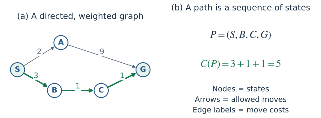
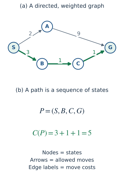
Figure 1. The graph determines what moves are possible and what they cost. The search algorithm decides which candidate to examine next; it does not redefine the objective.

1.2 An adjacency list is enough

For a small graph, a dictionary maps each state to a list of (neighbor, cost) pairs:

graph = {
    "S": [("A", 2), ("B", 3)],
    "A": [("G", 9)],
    "B": [("C", 1)],
    "C": [("G", 1)],
    "G": [],
}

def path_cost(graph, path):
    # This example has at most one directed edge between each pair.
    return sum(dict(graph[u])[v] for u, v in zip(path, path[1:]))

assert path_cost(graph, ["S", "A", "G"]) == 11
assert path_cost(graph, ["S", "B", "C", "G"]) == 5

zip(path, path[1:]) pairs each state with the next one: S–B, B–C, C–G. Looking up each edge’s cost and adding them computes the route cost; the last state has no following edge.

An adjacency list stores outgoing edges rather than a full matrix of all possible vertex pairs. A grid can generate these neighbors on demand; it does not need an explicit dictionary containing the whole map.

In graph["S"], ("A", 2) means “one allowed move reaches A and adds 2 to the route cost.” It does not mean that A has an intrinsic value of 2. The empty list for G means that G has no outgoing move, not that G is missing from the graph. graph.get(u, []) in later functions treats a missing key the same way.

A successor is a state reachable by one legal action. An explicit graph stores the successor lists; an implicit graph computes them. For a grid, a successor function tries the neighboring coordinates and rejects walls or out-of-bounds cells. For a puzzle, it applies the legal moves to the current configuration. Search needs the resulting (successor, cost) pairs, not a picture of the problem or a list of every state in advance.

1.3 The frontier is a collection of unfinished possibilities

Most search algorithms repeat the same broad operation:

1. Keep candidates in a frontier.
2. Remove one candidate according to a rule.
3. If it is the goal under the algorithm’s stopping rule, reconstruct the path.
4. Otherwise expand it: inspect its outgoing edges and add or update candidates.

Discovered means encountered and recorded. Expanded means selected for processing and its outgoing edges examined. A state can be discovered long before expansion, and in some algorithms it can be expanded more than once. “Visited” is too ambiguous to use as a correctness argument without saying which of these events it means.

The frontier is not the route taken by a moving character. It may simultaneously contain candidates from different branches. Expanding B after A does not assert that an edge A–B exists; it means that the computer has switched which unfinished candidate it is processing. The returned path must still follow the graph’s edges.

Path reconstruction uses a parent dictionary. If parent["C"] == "B", the currently recorded route reaches C from B. Starting at the goal and following parents gives the route backward:

def reconstruct(parent, goal):
    path = []
    node = goal
    while node is not None:
        path.append(node)
        node = parent[node]
    return path[::-1]

For a recorded route S → B → C → G, the parent entries are B: S, C: B, G: C, with S: None. Reconstruction visits G, C, B, S, stops at None, then reverses that list. The frontier says what remains to be processed; parent says how a recorded route reaches each state. These are different jobs even when the same dictionary also doubles as a discovered-state set.

path[::-1] is Python’s reversed-list slice. The snippets share definitions: DFS and BFS call this reconstruct helper, and later examples reuse earlier search functions. Running the downloadable notebook from top to bottom supplies those dependencies.

There is also a difference between the original graph and a search tree. A search-tree node represents a candidate route prefix: S → A → X and S → B → X are two tree nodes but end at the same graph state X. Plain graph DFS and BFS merge such repetitions by recording X once. Exhaustive path search keeps separate prefixes. This distinction explains why algorithms can inspect the same graph yet do very different amounts of work.

2. DFS: follow one branch before trying another

Depth-first search, DFS, uses a stack: the most recently added candidate is removed first. This is last in, first out, or LIFO. Put plates on a stack and the top plate is the first one available.

The following iterative graph search records each state when it is put on the stack. Reversing the neighbor list makes the first listed neighbor get popped first; it affects the route found, not reachability.

def dfs(graph, start, goal):
    stack = [start]
    parent = {start: None}  # Also records states already discovered.

    while stack:
        u = stack.pop()    # LIFO: follow the newest unfinished branch.
        if u == goal:
            return reconstruct(parent, goal)
        for v, _cost in reversed(graph.get(u, [])):
            if v not in parent:
                parent[v] = u
                stack.append(v)
    return None

assert dfs(graph, "S", "G") == ["S", "A", "G"]

Read the stack with its top on the right. Initially it is [S]. Popping S and appending B, then A, produces [B, A]. Popping A discovers G and produces [B, G]. G is then popped and accepted; B never needs to be expanded. The processing order is S, A, G, while the returned route is S → A → G. They happen to match here, but exploration order and a returned route are not generally the same list.

The test v not in parent marks discovery when pushing, so a cycle cannot keep adding the same state to this stack. This stack contains pending candidates, including sibling B, rather than exactly the current root-to-leaf route. A recursive DFS’s call stack retains its active ancestors. Both can find reachability, but their stack contents—and on graphs with cross-links, their recorded parent trees—need not be identical.

DFS finds a route on a finite graph if one exists, but the first route can be arbitrarily expensive. The code never compares edge costs. Changing the order of S’s neighbors can change its answer from cost 11 to cost 5 without changing the graph itself.

With adjacency lists and constant-time dictionary operations on average, this graph DFS takes $O(\lvert V\rvert+\lvert E\rvert)$ time and $O(\lvert V\rvert)$ auxiliary memory. Each state is pushed at most once and each reachable outgoing edge is inspected at most once. A recursive DFS uses the call stack instead; on a long chain that can exceed Python’s recursion limit.

The vertical bars count the members of a set: states for V and edges for E. Big-O notation describes how a resource requirement grows with input size, ignoring constant factors and lower-order terms. Linear in states plus edges does not mean a particular number of seconds; it means that the required work is bounded by a constant times that combined size once the input is large enough. Auxiliary memory excludes the already stored input graph.

2.1 Carve a maze: watch DFS build a tree

A maze can be a product of DFS rather than an input to it. Start with every room enclosed by walls. From the room at the top of the stack, choose an unvisited neighboring room, remove their shared wall, and push the new room. If every neighbor has already been visited, pop the stack and backtrack. A seed fixes the choices, so the same seed produces the same maze.

Carve a maze with DFS, then escape it

Controls

Loading interactive model…

Model & data

Randomized DFS generates an undirected rectangular maze; this phase constructs the graph rather than searching for a goal. It starts at cell (0,0), chooses an unvisited orthogonal neighbor uniformly from right/down/left/up candidates, removes the wall, and pushes the neighbor. With no unvisited neighbor it pops. A seeded 32-bit LCG makes every run reproducible. A completed N-cell maze has N−1 passages, is connected and has no cycles; each cell pair has one simple route. The player may walk through existing passages and undo. Counts exclude waiting, and the DFS stack is not the player's route. Seeds 0–999999, grids at most 7×5 in this UI. No score is stored or transmitted.

Before advancing, predict whether the next action will extend the corridor or return to an earlier junction. Compare seeds: which produces long corridors, and which backtracks early? The active stack is the unfinished branch; a room being popped is not an error or an abandoned solution, but a completed branch.

With $N$ rooms, carving always connects a new room to the visited region, so a finished maze has $N-1$ passages. It is connected and has no cycle: its passage graph is a spanning tree. There is exactly one simple route between any two rooms. Consequently, DFS and BFS on this finished maze must recover the same route, although their exploration effort can differ. Extra passages would create loops and give them different routes to choose from.

Maze generation and route search are different tasks. In generation, the algorithm creates edges between rooms; in route search, it must respect the edges already present.

In this lab the generator keeps the current room on the stack while it chooses just one new room. Its stack therefore really is the active route through the partly carved maze: popping returns to the previous room. Compare that with the earlier dfs function, which pops a candidate and pushes all of its unseen neighbors at once. The different stack displays reflect different implementations, not a conflict about LIFO.

2.2 N-Queens: reject a branch before it becomes a full board

Place one queen in each column of a chessboard, with no shared row or diagonal. A search state is not one square; it is a partial placement, such as [1, 3], meaning rows 1 and 3 in columns 0 and 1. A successor adds one queen in the next column.

The Python row and column indices start at zero; the lab numbers rows and columns from one in its messages and state readouts.

N-Queens: try a branch, prune, and backtrack

Controls

Loading interactive model…

Model & data

N=4, 5 or 6. A search state is a partial list of queen rows, one per consecutive column; rows and columns are shown from 1. Candidate rows are checked from top to bottom. Equal rows and equal absolute row/column differences conflict; one queen per column is built into the representation. Each step checks one candidate, records a complete solution, or returns from a completed branch. The solver starts from an empty board independently of manual placements and enumerates all solutions, counting rotations and reflections separately. A displayed solution is saved before the solver resumes backtracking. Saved-solution buttons pause the solver and display a complete placement without modifying its state or counts; Step/Run resumes an unfinished search. After enumeration the first saved solution remains on the board. Unsafe candidates are never expanded. No score or board state is persisted.

Try placing the queens yourself before starting the solver. When no safe row remains, remove the last queen and try another row. Then step the DFS solver and watch the same decision become a stack operation. A rejected placement is pruning: every extension would still contain the conflicting pair, so there is no reason to enumerate those full boards.

For queens in two distinct columns $i$ and $j$, write their row indices as $q_i$ and $q_j$. Every pair must satisfy

\[q_i\ne q_j,\qquad \lvert q_i-q_j\rvert\ne\lvert i-j\rvert.\]

The first condition excludes a shared row; the second excludes a shared diagonal. Columns are already distinct because the search adds exactly one queen per column. Every full solution has the same placement depth, so the purpose here is to find a feasible arrangement, not a cheaper route.

Try the pruning rule in Python

def can_place_queen(partial, row):
    col = len(partial)
    return all(row != old_row and abs(row - old_row) != col - old_col
               for old_col, old_row in enumerate(partial))

def queen_solutions(n, partial=()):
    if len(partial) == n:
        yield partial
        return
    for row in range(n):
        if can_place_queen(partial, row):
            yield from queen_solutions(n, partial + (row,))

assert can_place_queen((1, 3), 0)
assert not can_place_queen((1, 3), 2)
assert len(list(queen_solutions(4))) == 2

enumerate(partial) supplies each earlier queen’s column and row; all(...) requires every pair check to pass. (row,) is a one-element tuple, appended without changing the existing placement. yield emits one solution, and yield from passes on solutions from a recursive call. The function is a generator: list(...) collects its solutions before len(...) counts them.

Why is row 2 forbidden after (1, 3)? It shares a diagonal with the queen in column 1, row 3. A global “visited square” set would not represent this problem: whether a square is safe depends on the whole partial placement.

3. BFS: explore one distance layer at a time

Breadth-first search, BFS, replaces the stack with a queue: the oldest candidate is removed first. This is first in, first out, or FIFO. Everyone who entered the queue before you is served before you.

from collections import deque

def bfs(graph, start, goal):
    queue = deque([start])
    parent = {start: None}

    while queue:
        u = queue.popleft()  # FIFO: finish the older distance layer first.
        if u == goal:
            return reconstruct(parent, goal)
        for v, _cost in graph.get(u, []):
            if v not in parent:
                # Mark on enqueue, not on dequeue: avoid duplicate entries.
                parent[v] = u
                queue.append(v)
    return None

assert bfs(graph, "S", "G") == ["S", "A", "G"]

A Python list’s pop(0) shifts the remaining elements. deque.popleft() removes the front element without that linear shift.

Read this queue from the left, where removal happens. On the same graph, expanding S gives [A, B]; expanding A gives [B, G]; expanding B gives [G, C]. G is removed next, so the result is still S → A → G. BFS does not prefer A’s cost 2 to B’s cost 3: it processes A first because S listed A first. It accepts the goal before C because G was reached in two moves, while reaching G through C would take three.

Recording discovery on enqueue is important when branches meet. Suppose A and B both lead to X. If A enqueues X first, B must not enqueue it again while X is waiting. The parent entry already records that first discovery. Without that check, the queue could hold many copies of the same state even before any copy is removed. With unit costs, the first entry is already sufficient for a shortest route.

3.1 Why does BFS find the fewest edges?

Define the depth of a state as the number of edges in a shortest route from the start. The queue initially contains only depth zero. Expanding a depth-$d$ state generates depth-at-most-$d+1$ candidates, which are added behind all older candidates. Consequently, the queue processes states in nondecreasing shortest depth. The first discovery of a state already gives a minimum-edge-count route to it.

If every edge costs the same positive amount $a$, then

\[C(P)=a\,k(P), \tag{3}\]

so minimizing the number of edges also minimizes cost. If all edges have cost zero, every reachable path has cost zero as well. With unequal edge costs, the depth argument remains valid but no longer proves minimum cost.

Like DFS, graph BFS takes $O(\lvert V\rvert+\lvert E\rvert)$ time and $O(\lvert V\rvert)$ auxiliary space on a finite explicit graph. On an implicit search tree with branching factor $b$ and shallowest goal depth $d$, the number of states through that depth is about

\[\begin{gathered} 1+b+b^2+\cdots+b^d=O(b^d),\\ b>1. \end{gathered} \tag{4}\]

There is no contradiction: the implicit state space itself can grow exponentially with depth. BFS’s broad frontier makes memory a practical limitation.

Here the branching factor is the number of successors per search-tree node in the simplified full-tree count. Two choices at each step give 1 candidate at depth zero, 2 at depth one, 4 at depth two, and so on. A real graph can merge branches or have fewer successors; the formula explains the potential growth, not an exact count for every map. The visible BFS frontier is the waiting boundary between processed layers and layers not yet reached.

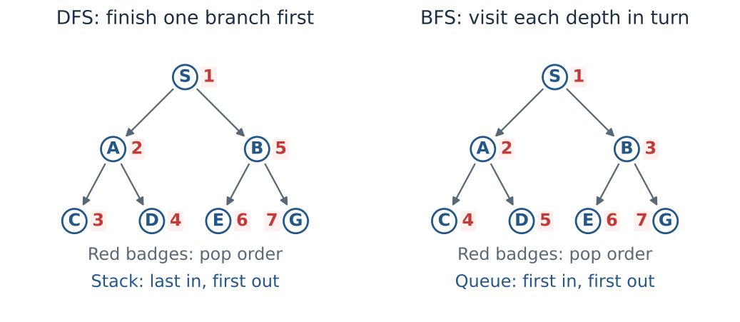
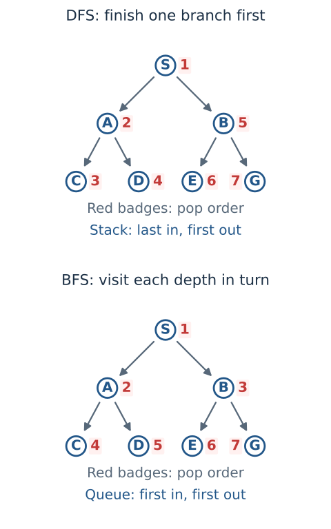
Figure 2. Red badges show the order in which candidates are removed, with a left-to-right neighbor preference. Arrows are graph edges, not successive steps of the exploration. This seven-state tree is a separate example from the five-state graph in the code.

DFS and BFS: inspect the frontier

Controls

Loading interactive model…

Model & data

Finite 13×9 authored grid. Four-direction movement, unit edge costs, neighbor order right/down/left/up. DFS uses a stack and BFS a queue; both mark states discovered when inserted. Goal detection occurs when removed from the frontier. Expanded counts states whose successors were examined; the goal is not expanded. Frontier and peak count distinct active states. Colors and letters distinguish frontier, expanded, current and final path.

Try Step several times with DFS, reset, and repeat with BFS. Predict the next candidate before pressing the button. Then compare the returned route with the number of expanded states. A shorter route does not necessarily require fewer expansions.

Quick quiz: can BFS stop when it discovers the goal?

Yes, for this ordinary unweighted BFS. The first discovery gives the shortest depth. The code above checks on removal to keep its structure easy to compare with later algorithms. For Dijkstra and A*, stopping on first discovery is generally wrong: a cheaper route may still be waiting in the frontier.

3.2 Word ladder: a graph with no map coordinates

Change COLD into WARM, changing one letter at a time and using only words in the displayed dictionary. A word is a state; an edge joins words that differ at exactly one position. Each change costs one. The dictionary is the exact allowed state set, not a request to guess which words a real-world dictionary might accept.

Word ladder: change COLD into WARM

Controls

Loading interactive model…

Model & data

A finite authored dictionary is the complete vertex set, not a claim about all English words. An undirected edge joins two words of equal length if exactly one letter differs; each edge costs 1. Click a legal neighbor to build your chain. BFS uses alphabetically ordered neighbors, marks states when enqueued, and checks the goal when dequeued. Layers show discovered words by their shortest distance from the start; blue words are queued and gray words have had successors examined. The manual chain and the BFS demonstration are independent. Each manual attempt is capped at 40 moves. No score is stored or transmitted.

Build a chain by choosing a legal next word. Can you reach the goal without revisiting a word? Compare your chain with the BFS route and inspect its distance layers. A word that resembles the goal is not necessarily on the shortest ladder: it may connect to the wrong part of the dictionary.

For the default COLD → WARM puzzle, a four-change route is COLD → CORD → CARD → WARD → WARM. All four letter positions differ between the endpoints, so any valid route needs at least four changes. This route reaches that lower bound. The HEAD → TAIL preset needs a detour: all four positions differ, but its shortest chain uses five changes. Removing a necessary intermediate word can also make a word ladder unsolvable.

Build word-graph edges with Python

ladder_words = ("COLD", "CORD", "CARD", "WARD", "WARM",
                "WORD", "WORM", "BOLD")
word_graph = {
    word: [(other, 1) for other in ladder_words
           if sum(a != b for a, b in zip(word, other)) == 1]
    for word in ladder_words
}
ladder = bfs(word_graph, "COLD", "WARM")
assert len(ladder) - 1 == 4

This small dictionary is sufficient for the example route. The browser lists its complete dictionary for each preset. Replacing the vocabulary changes the graph, even if the start and goal stay the same.

3.3 Water jugs: search over quantities instead of places

Two jugs hold at most 3 and 5 liters. Starting with both empty, obtain exactly 4 liters in either jug. Each action fills one jug, empties one jug, or pours one jug into the other until the source is empty or the destination is full. An action that changes nothing is omitted. All remaining actions cost one.

Water-jug puzzle: measure exactly 4 liters

Controls

Loading interactive model…

Model & data

A state (a,b) records integer liters in jugs A and B. Start (0,0); the goal is exactly the target amount in either jug. Six action types are allowed: fill either jug completely from an unlimited tap, empty either jug completely to a drain, or pour in either direction until the source empties or the destination fills. No intermediate stopping or scale marks may be used. Every nontrivial action costs 1, independent of liters moved; unchanged actions are omitted. BFS explores this finite directed state graph in the listed action order, discovers on enqueue and tests on dequeue. The 2L/4L target3L preset is deliberately unreachable. Manual play and the BFS trace are independent, and each manual attempt is capped at 40 actions. No state or score leaves the page.

Try the controls yourself and count actions before revealing BFS’s solution. The state is the pair of current amounts, not the last button pressed. A fill action can add several liters yet still be one edge, so BFS minimizes actions, not liters moved or water consumed.

For capacities $A$ and $B$, the state space is contained in

\[\{0,1,\ldots,A\}\times\{0,1,\ldots,B\}.\]

Only 24 pairs are possible for the 3-liter/5-liter puzzle, and fewer may be reachable. If the current amounts are (a, b), a pour from the first jug to the second transfers

\[\begin{gathered} \delta=\min(a,B-b),\\ (a,b)\longrightarrow(a-\delta,b+\delta). \end{gathered}\]

This successor rule enforces both capacity and conservation during a pour. Filling and emptying exchange water with the tap or drain and therefore do not conserve the total amount in the two jugs.

One shortest solution, and a puzzle with no solution

The default puzzle needs six actions: fill the 5-liter jug, pour into the 3-liter jug, empty the 3-liter jug, pour the remaining two liters into it, fill the 5-liter jug again, then pour one liter into the 3-liter jug. The final amounts are (3, 4).

For capacities 2 and 4 with an odd target, no sequence of these actions can work: all reachable quantities remain multiples of 2. The lab can exhaust its finite frontier and show failure rather than continue trying forever. This is a statement about the allowed full-fill/full-empty/full-pour actions; permitting arbitrary partial pours would define a different problem.

4. Brute force is not the same thing as DFS

Brute force describes an exhaustive strategy, not a particular container. One brute-force shortest-path method enumerates every simple start-to-goal path, computes its cost, and keeps the cheapest. A simple path does not repeat a state.

On a finite graph with nonnegative costs, at least one optimal route, if a route exists, is simple: removing a cycle cannot increase its cost. That justifies restricting enumeration to simple paths. It does not justify ignoring a state globally after seeing it on one path; different paths may reach it at very different costs.

def exhaustive_shortest(graph, start, goal):
    best_path, best_cost = None, float("inf")

    def visit(u, path, cost):
        nonlocal best_path, best_cost
        if u == goal:
            if cost < best_cost:
                best_path, best_cost = path[:], cost
            return
        for v, edge_cost in graph.get(u, []):
            if v not in path:  # Path-local cycle check, not a global seen set.
                visit(v, path + [v], cost + edge_cost)

    visit(start, [start], 0)
    return best_path, best_cost

assert exhaustive_shortest(graph, "S", "G") == (["S", "B", "C", "G"], 5)

nonlocal lets the nested visit function update the enclosing function’s best_path and best_cost. path[:] copies a completed route, and path + [v] creates a new list for the next branch. Each recursive call therefore has its own candidate path rather than changing one list shared by every branch.

This code traverses the tree of candidate paths in a depth-first order, yet does much more work than the graph DFS above. A state can appear in many distinct candidate paths. In a complete directed graph, every pair of distinct vertices has an edge in each direction. The number of simple paths between two distinct fixed endpoints is

\[\sum_{j=0}^{\lvert V\rvert-2}\frac{(\lvert V\rvert-2)!}{(\lvert V\rvert-2-j)!}, \tag{5}\]

because we can choose and order any subset of the other vertices. Even a small increase in graph size can make enumeration impractical. The recursion is useful as a small independent reference, not as the main route planner.

Here $j$ counts intermediate vertices, excluding the fixed start and goal. The ! symbol means factorial, such as 3! = 3 × 2 × 1, with 0! = 1. In a complete graph with five vertices, choosing zero, one, two or three intermediate vertices gives 1 + 3 + 6 + 6 = 16 simple routes between fixed distinct endpoints. The factorials count the different orders as well as the choices of intermediate vertices.

The improvement we need is not merely to “try cleverer routes first.” We should also avoid solving the same remaining problem separately for every prefix of a path. If future options depend only on the current state, a cheaper route to that state dominates a more expensive one.

For example, suppose two prefixes reach X with costs 4 and 9. Any continuation from X that costs another 6 gives complete routes of cost 10 and 15. The same five-unit disadvantage remains for every common continuation. Keeping the cheaper prefix is therefore enough for finding the minimum cost; keeping both only repeats the remaining work. This is dominance, and it is the reason to store a best cost for each state rather than every route to it.

That argument requires the two prefixes to leave the same future options. Arriving at X without a key and arriving with it are not interchangeable, even if one is cheaper. They must be different states. Likewise, if a rule forbids reusing a resource, the state must record whether that resource has already been used. A good state definition is what makes safe duplicate elimination possible.

5. Unequal costs: why BFS fails and relaxation matters

In the running graph, the two relevant routes are

\[S\to A\to G:\quad 2+9=11,\] \[S\to B\to C\to G:\quad 3+1+1=5.\]

BFS returns the two-edge route. It is correct about edge count and wrong about the minimum-cost objective. Calling all graph algorithms “shortest-path algorithms” without specifying what length means hides this distinction.

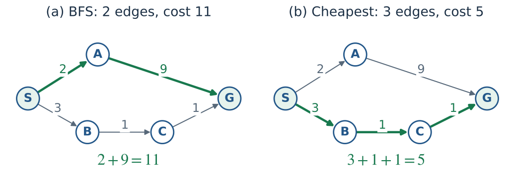
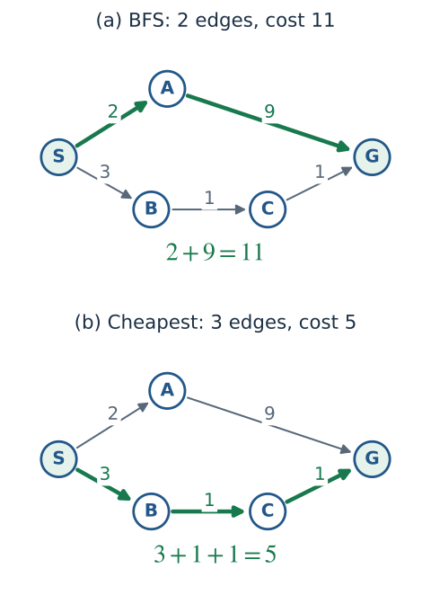
Figure 3. The cheaper route has more edges. Both algorithms must be judged against the same sum-of-costs objective.

Let $g(v)$ be the cost of the cheapest route to $v$ found so far. This is a recorded upper bound on the true minimum cost to $v$, not a prediction:

\[\begin{aligned} g(s)&=0,\\ g(v)&=\infty\quad(v\ne s)\text{ initially}. \end{aligned} \tag{6}\]

“Upper bound” means that a discovered route provides a cost we can actually achieve, so the unknown optimum cannot be larger than that recorded route cost. Before finding any route to a state, infinity is a sentinel meaning “no finite route known yet,” not a very large physical movement cost. It does not prove the state unreachable. In the implementation, best_g.get(v, float("inf")) supplies this initial value without storing every state in advance.

When we expand $u$, each edge offers a candidate route to $v$:

\[g_{\mathrm{candidate}}(v)=g(u)+c(u,v).\]

If it is cheaper, we update both the cost and the parent:

\[\begin{gathered} \text{if }g(u)+c(u,v)<g(v):\\ \begin{aligned} g(v)&\leftarrow g(u)+c(u,v),\\ \operatorname{parent}(v)&\leftarrow u. \end{aligned} \end{gathered} \tag{7}\]

This operation is called relaxation. The strict inequality matters: replacing an equal-cost route is unnecessary for cost optimality and can repeatedly circulate through zero-cost cycles.

In the running graph, expanding A offers G a route costing 2 + 9 = 11, so its cost changes from infinity to 11 and its parent becomes A. Later, expanding C offers 4 + 1 = 5. Five is smaller, so G’s cost becomes 5 and its parent becomes C. Updating only the number would leave reconstruction following the wrong route. Relaxation updates both records, but by itself does not decide which state should be expanded next; that is the frontier’s ordering rule.

6. Dijkstra: expand the smallest known cost

Dijkstra’s algorithm, also called uniform-cost search when used for a goal-directed search, orders the frontier by $g$. A priority queue removes the entry with the smallest numeric priority, regardless of insertion time. A binary min-heap implements insertion and removal in logarithmic time.

BFS’s FIFO order answers “which candidate was discovered first?” Dijkstra instead asks “which recorded route costs least?” The change is necessary because a later discovery can be cheaper. A heap lets that cheaper entry move ahead of older, more expensive entries without sorting the entire frontier after every insertion.

from heapq import heappush, heappop
from itertools import count

def dijkstra(graph, start, goal):
    serial = count()  # A unique tie-breaker; nodes need not be comparable.
    heap = [(0, next(serial), start)]
    best_g = {start: 0}
    parent = {start: None}

    while heap:
        g_entry, _order, u = heappop(heap)
        if g_entry != best_g[u]:
            continue  # A newer, cheaper entry superseded this one.
        if u == goal:
            return reconstruct(parent, goal), g_entry

        for v, edge_cost in graph.get(u, []):
            if edge_cost < 0:
                raise ValueError("Dijkstra needs nonnegative edge costs")
            candidate = g_entry + edge_cost
            if candidate < best_g.get(v, float("inf")):
                best_g[v] = candidate
                parent[v] = u
                heappush(heap, (candidate, next(serial), v))
    return None, float("inf")

assert dijkstra(graph, "S", "G") == (["S", "B", "C", "G"], 5)

The graph is assumed to contain finite costs. The check inside the loop catches encountered negative edges; it is not a full prevalidation of a graph that may terminate before inspecting every edge.

Each heap entry is (cost, serial, state). Python compares tuples from left to right: cost determines the priority; a unique increasing serial breaks cost ties by insertion order. It also prevents Python from trying to compare arbitrary state objects. g_entry is the cost saved when that entry was pushed, whereas best_g[u] is the most recent recorded cost. Their difference identifies an obsolete entry. The variable _order receives the serial but is not otherwise used.

The following trace uses exactly the earlier graph. Queue entries are displayed in increasing removal order, with the serial omitted; the table is not the heap’s internal array.

Valid removal	Update made	Queue after processing
S, cost 0	A gets 2; B gets 3	A:2, B:3
A, cost 2	G gets 11, parent A	B:3, G:11
B, cost 3	C gets 4	C:4, G:11
C, cost 4	G improves to 5, parent C	G:5, G:11 (old)
G, cost 5	Accept goal; reconstruct	G:11 remains unused

G is discovered before C, but C is processed first because 4 is less than 11. After the improvement, the queue holds two records for G; there is still only one current best_g["G"], equal to 5. Following the final parents backward gives G ← C ← B ← S, hence the cost-5 answer.

6.1 Why is removal the right stopping time?

Let $g^{\ast}(v)$ denote the true minimum cost from $s$ to $v$. Dijkstra’s invariant is that, when a non-stale entry is removed with minimum $g$, its cost equals $g^{\ast}(v)$.

Such a state is called settled: its recorded cost is now final. Before removal its number is tentative, even if it already appears beside the state in a diagram. The claim is stronger than “this is the cheapest entry currently visible”: nonnegative edge costs ensure that no route still waiting to be developed can later improve it.

Suppose the removed state $u$ had a cheaper route that we had not completed. Along that route there would be a first not-yet-settled state $x$ whose predecessor was settled. Expanding that predecessor would already have generated an entry for $x$ with cost no larger than the cheap route to $u$, because all remaining edge costs are nonnegative. That entry would have to be removed before $u$, contradicting the choice of $u$.

Thus the goal is safe to accept when its valid minimum-cost entry is removed—not when any edge first reaches it. In the running example, expanding A discovers the goal at cost 11. B and C still lead to a better entry at cost 5.

6.2 Why are old heap entries left in place?

Python’s heapq has no direct decrease-key operation. If a state’s cost improves from 11 to 5, we push a new entry and leave the old entry in the heap. When the old entry eventually appears, its stored cost no longer matches best_g and it is discarded. This is lazy deletion, a standard priority-queue pattern described in the Python heap documentation.

The array backing a heap is not a fully sorted list. Only the minimum is guaranteed at its root. A displayed frontier sorted for readability is therefore a view of the queue, not its internal array layout.

6.3 Plan a delivery: fewer roads, more minutes

Eight stops are joined by roads whose labels give travel times in minutes. The direct A–H road takes 18 minutes. The upper A–B–C–H route takes 12. The lower A–D–E–F–G–H route takes 10, despite using more roads. Coordinates only arrange the drawing; they do not determine travel time.

Delivery challenge: few roads or few minutes?

Controls

Loading interactive model…

Model & data

Eight authored stops, eleven positive undirected roads. Labels are fixed minutes, not geometric distance. Deliver A→H by clicking connected stops. Normal: direct A–H=18; A–B–C–H=12; A–D–E–F–G–H=10. Traffic multiplies A–D, D–E, E–F, F–G and G–H by 3; other presets close E–F or all H roads. Changes restart the search. One Step removes one raw priority-queue entry; an obsolete entry is discarded without relaxation. Valid pops settle a stop, then examine all its neighbors. Delivery ends on a valid minimum-g goal pop, not discovery. Ties use source ID, stop ID, then insertion order. Manual routes may revisit stops; only open connected roads are legal. No score is saved.

Click connected stops to plan your delivery before comparing with Dijkstra. Then introduce traffic or close a bridge. Does the route you chose remain optimal? A route can remain legal after traffic changes while becoming more expensive than an alternative. With the lower roads tripled in cost, the upper route wins at 12 minutes. Closing E–F also makes a 12-minute route optimal; isolating H makes delivery impossible.

During the solver trace, distinguish “H has a number next to it” from “H has been removed as the cheapest valid candidate.” The first is only a discovered route; the second is the certificate needed to stop.

The route you click and the solver’s search are separate: the former is one proposed delivery, while the frontier may represent several competing deliveries at once. Read the road labels as individual costs and the node labels as accumulated costs from A. Their units are both minutes, but they answer different questions. After changing traffic or a closure, restart the search because its old tentative costs described the previous road network.

6.4 Dispatch from two stations: one search, several starting points

An emergency at E may be served from A or H. We need the quickest arrival from either station, not a route that visits both. Initialize each station with cost zero in the same priority queue. Ordinary relaxation then propagates the cheapest arrival label, along with the station that supplied it. Write $\mathcal S$ for the station set, and $d(s,v)$ for the minimum travel time from $s$ to $v$:

\[d_{\mathcal S}(v)=\min_{s\in\mathcal S}d(s,v).\]

Dispatch desk: two stations, one shared frontier

Controls

Loading interactive model…

Model & data

The same eight-stop positive undirected network, with two distinct stations initialized at g=0 in one priority queue. Dijkstra runs until the queue is exhausted, finding min(dist(station1,v),dist(station2,v)) at every reachable v. Both stations start immediately; no capacity, congestion caused by vehicles, service duration or waiting-time model is included. On equal arrival time the alphabetically earlier source wins; a queue entry is stale if either its distance or owner is obsolete. Coloring before settlement is tentative; a square ring marks a station and a solid circle outline marks settled stops. Select any emergency stop, or move either station. Presets include A+H, A+G (a four-minute tie at E), and B+F. Changing stations or road conditions restarts both wavefronts.

Change the stations or road conditions and predict which station will reach the selected stop first. With stations at A and H on the default network, E is four minutes from A and F is four minutes from H. With stations A and G, E is tied at four minutes; the displayed owner uses a deterministic tie rule, not a claim that one station is genuinely faster.

This is multi-source Dijkstra. A station can serve many destinations; the demo has no vehicle capacity, dispatch scheduling, or competition between simultaneous emergencies. Its task is an earliest-arrival distance calculation.

Use a virtual super-source with the existing Python function

roads = [("A", "H", 18), ("A", "B", 4), ("B", "C", 4), ("C", "H", 4),
         ("A", "D", 2), ("D", "E", 2), ("E", "F", 2), ("F", "G", 2),
         ("G", "H", 2), ("B", "E", 3), ("C", "F", 3)]
town = {name: [] for name in "ABCDEFGH"}
for u, v, minutes in roads:
    town[u].append((v, minutes))
    town[v].append((u, minutes))

super_source = object()
dispatch_graph = {u: edges[:] for u, edges in town.items()}
dispatch_graph[super_source] = [("A", 0), ("H", 0)]
assert dijkstra(town, "A", "H")[1] == 10
assert dijkstra(dispatch_graph, super_source, "E")[1] == 4
assert dijkstra(dispatch_graph, super_source, "F")[1] == 4

The zero-cost virtual edges encode the initial condition; they are not physical roads. The browser directly inserts both stations at zero, which is equivalent and avoids creating an extra vertex.

7. A heuristic: a lower-cost problem hiding inside the real one

A heuristic $h(n)$ estimates the minimum cost still needed to get from $n$ to the goal. It is not learned automatically by A*. Someone must derive, calculate, or supply it.

Dijkstra can compare the prices of routes already found, but those prices say nothing about which candidate is nearer the destination. A heuristic supplies that missing goal information. It answers a different question from best_g: not “how cheaply have I reached this state?” but “how much more might reaching the goal require?” For a fixed goal, the heuristic can be a small function of the state. The search calls that function when needed; it does not have to solve a new shortest-path problem at each call.

The distinction also explains why the two values change differently. A newly discovered route can improve the recorded cost of reaching the same state. Its heuristic stays the same because the state, goal, and remaining movement rules have not changed. A heuristic is measured in the same cost units as the route objective, not in probability or confidence.

On a four-direction grid, removing all walls and setting every step cost to a global lower bound $a$ gives an easier problem. If each real horizontal or vertical step costs at least $a$, the shortest route in this uniform-cost relaxed grid from $(x,y)$ to $(x_t,y_t)$ costs

\[\begin{aligned} h_{\mathrm{Manhattan}}(n) &=a\bigl(\lvert x-x_t\rvert\\ &\qquad+\lvert y-y_t\rvert\bigr). \end{aligned} \tag{8}\]

Why is it a lower bound? A legal route must correct the horizontal displacement and the vertical displacement. Each orthogonal move changes only one coordinate by one. Walls can force extra steps but cannot make those required coordinate changes disappear.

This is a relaxed problem: remove constraints without making retained moves more expensive. Its exact optimum is a lower bound on the constrained optimum. That construction is often more reliable than inventing a number that merely “looks close.” Berkeley’s informed-search notes explain heuristics through the same relaxation principle.

For example, take a state at column 2, row 1 and a goal at column 6, row 4. With four-direction movement, at least four horizontal and three vertical moves are necessary. If every move costs at least 2, the relaxed answer is 14. A wall might make the cheapest legal route cost 18, but it cannot reduce the cost below 14. Computing 14 needs only the coordinates and the minimum step price; discovering the actual cost 18 requires searching around the wall. This gap is precisely what makes a useful heuristic cheaper to compute than the answer it helps find.

7.1 Greedy best-first search uses only the estimate

Greedy best-first search orders candidates by

\[f_{\mathrm{greedy}}(n)=h(n). \tag{9}\]

It can move rapidly toward the destination, but ignores how much it has already spent. A state that looks close may have been reached through a very expensive corridor.

For the running graph, choose the fixed heuristic values

\[\begin{aligned} h(S)&=3,\quad h(A)=1,\\ h(B)&=2,\quad h(C)=1,\\ h(G)&=0. \end{aligned}\]

These values are lower bounds on remaining cost and even satisfy consistency, defined below. Greedy nevertheless chooses A before B, then G before B, and returns cost 11. A good heuristic does not make an algorithm that ignores $g$ cost-optimal.

Candidate after expanding S	$g$	$h$	Dijkstra: $g$	Greedy: $h$	A*: $g+h$
A	2	1	2	1	3
B	3	2	3	2	5

Both Dijkstra and A* also expand A before B here. The crucial difference is what happens after G is discovered from A. Greedy gives G priority zero; A* gives it priority 11 and keeps searching lower-priority alternatives first.

“Ignoring the cost already spent” refers to each candidate’s own route, not to one traveler physically walking around the graph. Search retains competing routes at the same time. After examining A, it can still select the route ending at B without paying to walk back from A. Greedy sees only that G has no distance left to travel; it does not compare the cost-11 route to G with the unfinished cost-3 route to B.

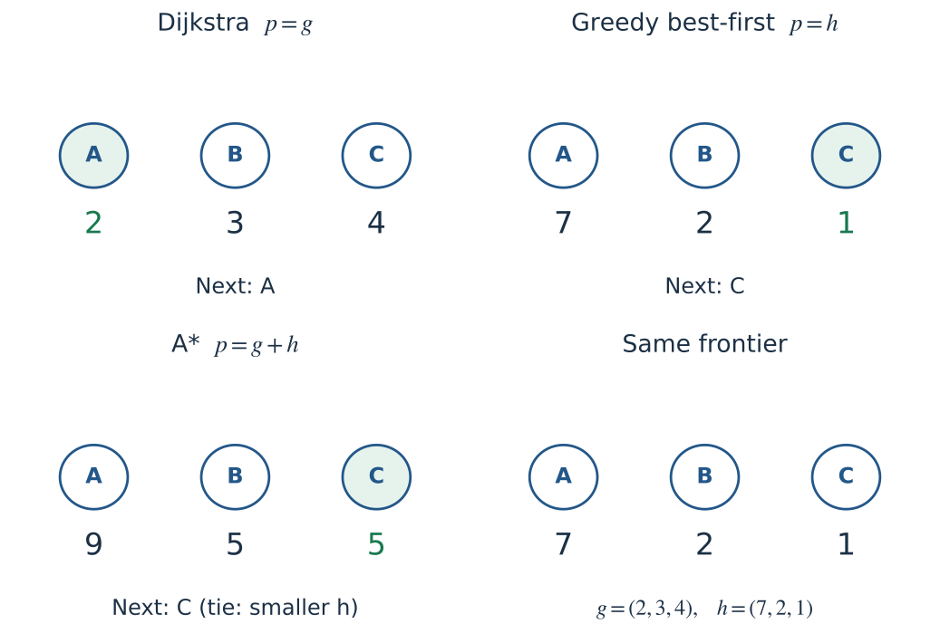
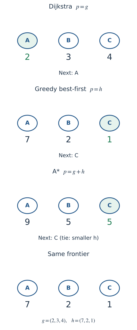
Figure 4. A separate illustrative frontier with three candidates, not the two-candidate frontier in the table above. Dijkstra picks A; greedy and A* pick C. B and C tie at $g+h=5$, and the smaller-$h$ tie-break favors C. A heuristic changes the ordering, not the objective or the relaxation step.

8. A*: combine what is known with what remains

A* uses

\[f(n)=g(n)+h(n). \tag{10}\]

$g(n)$ is the actual cost of a specific discovered prefix. $h(n)$ estimates the best possible suffix. Their sum estimates the cost of a complete route through that prefix. It need not equal the cost of any feasible complete path: the heuristic may ignore obstacles.

Setting $h\equiv0$ makes A* use the same primary priority as Dijkstra. With identical tie handling, the two algorithms have the same behavior. A* is therefore not a completely separate search mechanism; it is a goal-informed priority rule built on relaxation.

The sum evaluates a particular candidate route, not the state in isolation: keep its currently recorded prefix, then estimate the cheapest continuation. It is not the straight-line distance from the start, and it is not necessarily the price of a complete route already found. Selecting its smallest value means investigating the most promising unfinished candidate, not committing to follow that route to the end.

The running graph gives a complete small trace. In the table, each triple lists (g, h, f); only the newest valid entry for each state is shown.

After this expansion	Valid frontier entries	Next removal
None	S (0, 3, 3)	S
S	A (2, 1, 3); B (3, 2, 5)	A
A	B (3, 2, 5); G (11, 0, 11)	B
B	C (4, 1, 5); G (11, 0, 11)	C
C	G (5, 0, 5)	G: return cost 5

A* still tries A first; the heuristic need not predict the correct branch immediately. What matters is that the expensive goal candidate does not end the search while cheaper-priority unfinished candidates remain. Expanding C replaces G’s recorded prefix with the cost-5 route. A heap implementation may retain the obsolete cost-11 entry internally, but that entry no longer represents the best recorded route.

8.1 Admissibility: do not overestimate the remaining optimum

Write $h^{\ast}(n)$ for the true cheapest remaining cost from $n$ to $t$. A nonnegative heuristic is admissible if

\[\begin{gathered} 0\le h(n)\le h^{\ast}(n),\\ h(t)=0. \end{gathered} \tag{11}\]

For a state from which the goal is unreachable, $h^{\ast}(n)=\infty$, so a finite heuristic does not violate this condition. For a reachable state, overestimating may cause A* to postpone the only cheap route until after it accepts an expensive goal.

Do not confuse this with the recorded $g(n)$. Since $g(n)$ is the cost of an actual route, it normally satisfies $g(n)\ge g^{\ast}(n)$. The two terms bound different unknowns in opposite directions.

Here $g^{\ast}(n)$ means the true cheapest cost from the start to the state, while $h^{\ast}(n)$ means the true cheapest cost from the state to the goal. The stars indicate unknown optimal values, not extra quantities that A* must already have computed. best_g stores the best prefix found so far; the supplied heuristic estimates the suffix.

Consequently, admissibility does not make every current $f(n)$ a lower bound on the globally optimal answer. Suppose a state’s recorded prefix costs 8 although its best possible prefix costs 4, and its heuristic is 2 although its true remaining cost is 3. The current estimate is 10, while the cheapest route through that state costs 7. The heuristic has not overestimated anything; the recorded prefix is simply not optimal yet. The optimality proof needs a frontier entry with an optimal prefix, not an arbitrary frontier entry.

8.2 Why admissible A* returns an optimal path

Assume a finite graph, nonnegative finite edge costs, an admissible fixed heuristic, and reopening whenever a cheaper route is found. Stop when a valid goal entry is removed from the priority queue.

If an optimal route has not yet been completed, there is a frontier entry $n$ on an optimal route whose recorded prefix cost is already optimal. This frontier entry exists because expanding its optimal predecessor relaxes the next edge; reopening allows that argument to remain true even when a state was expanded earlier through a worse prefix.

To see why such an entry cannot disappear, fix one optimal route and follow it from the start. Initially its start entry has the correct cost zero. Whenever a state on this route is expanded with its optimal prefix cost, relaxation offers the next state the optimal cost too. That next state is either waiting in the frontier, or has already been expanded at that cost and has passed the same opportunity onward. Before the optimal goal has been removed, some part of this progression must still be waiting. Every prefix of an optimal route is itself optimal: replacing a prefix by a cheaper one would give a cheaper complete route. Reopening is what keeps this progression available if an intermediate state was processed earlier at a worse cost.

For this entry,

\[\begin{aligned} f(n)&=g^{\ast}(n)+h(n)\\ &\le g^{\ast}(n)+h^{\ast}(n)\\ &=C^{\ast}. \end{aligned} \tag{12}\]

If A* tried to remove a goal with cost $C>C^{\ast}$, its priority would be $C+h(t)=C$. But the frontier still contains an entry with priority at most $C^{\ast}$, which must be selected first. This contradiction proves that the returned goal cost is $C^{\ast}$.

Two implementation details carry the proof. The goal estimate is zero, so a goal’s priority equals its actual recorded route cost. Also, “removed” means the smallest valid queue entry, not the moment an edge first discovers the goal. Discovery leaves cheaper-priority alternatives in the frontier, exactly as the cost-11 goal did in the trace above.

The proof does not say that every expanded state had its optimal prefix cost. That stronger property needs consistency. Nor does it say A* explores only the final path; a lower bound can be optimistic about routes that later become dead ends.

Why finite graphs and strict updates matter

With a finite graph and nonnegative costs, strict improvements prevent endless equal-cost updates around zero-cost cycles. The algorithms can exhaust all reachable candidates and report no route. In an infinite state space, completeness needs additional assumptions—commonly finite branching and a positive lower bound $\epsilon$ on step cost, so only finitely many relevant paths fit under a finite cost threshold. A finite-grid demo is not a proof of termination in every infinite planning problem.

9. Consistency and the reason some states must be reopened

An admissible heuristic compares each state with a potentially distant goal. Consistency adds a local condition for every directed edge:

\[\begin{gathered} h(u)\le c(u,v)+h(v),\\ h(t)=0. \end{gathered} \tag{13}\]

The estimate at $u$ must not exceed the cost of taking one legal step plus the estimate after that step. This resembles the triangle inequality. Applying it repeatedly along any route to the goal proves $h(u)\le C(u\leadsto t)$; taking the minimum gives admissibility.

The two conditions test different comparisons. Admissibility compares one estimate with the entire true remaining journey, which may be expensive to compute. Consistency compares estimates at neighboring states using one known edge cost. For example, if an edge costs 1 and the next state’s estimate is 0, consistency permits an estimate of at most 1 before that edge. A value of 4 would violate consistency even if the actual remaining journey still costs 4 or more. An estimate can be safe relative to the destination yet change too abruptly across one edge.

On a particular discovered route, $g(v)=g(u)+c(u,v)$, so

\[\begin{aligned} f(v)-f(u)&=c(u,v)\\ &\quad+h(v)-h(u)\\ &\ge0. \end{aligned} \tag{14}\]

Thus priorities cannot decrease as that route is extended. Consistent A* settles each state on its first valid expansion, and a permanent closed set is safe. With an admissible but inconsistent heuristic, a state may need to be expanded again at a better cost.

9.1 A four-state counterexample

Use these directed edges:

\[\begin{gathered} S\to A:3,\quad S\to B:1,\\ B\to A:1,\quad A\to G:3,\\ B\to G:100. \end{gathered}\]

The optimum is $S\to B\to A\to G$ with cost 5. Choose

\[\begin{aligned} h(S)&=5,\quad h(A)=0,\\ h(B)&=4,\quad h(G)=0. \end{aligned}\]

Every value is admissible: the true remaining costs are 5, 3, 4, and 0. But the edge $B\to A$ violates consistency because $4>1+0$.

After expanding S, A has $(g,f)=(3,3)$ and B has $(1,5)$. A is expanded first and generates G with cost 6. B is then expanded and finds a cheaper route to A, with $g(A)=2$. If A is permanently closed, that improvement cannot propagate through A to G and the algorithm returns 6. Reopen A and its new priority 2 leads to the correct goal cost 5.

The decrease in priority does not mean walking along an edge refunds past expenditure. Extending the route from B to A increases its prefix cost from 1 to 2. The priority falls from 5 to 2 because the heuristic drops from 4 to 0 across an edge costing only 1. Separately, the newly found prefix to A costs 2 instead of the previously recorded 3. These are two different comparisons: extending one route, and replacing an older route to the same state.

Reopening therefore requires more than changing A’s displayed number. Set A’s best cost to 2, change its parent from S to B, and put it back in the frontier. Expanding it again offers G the improved cost 5, changes G’s parent record if needed, and inserts a new goal candidate. Updating only the cost would leave path reconstruction inconsistent; updating the parent without expanding again would fail to carry the saving to later states.

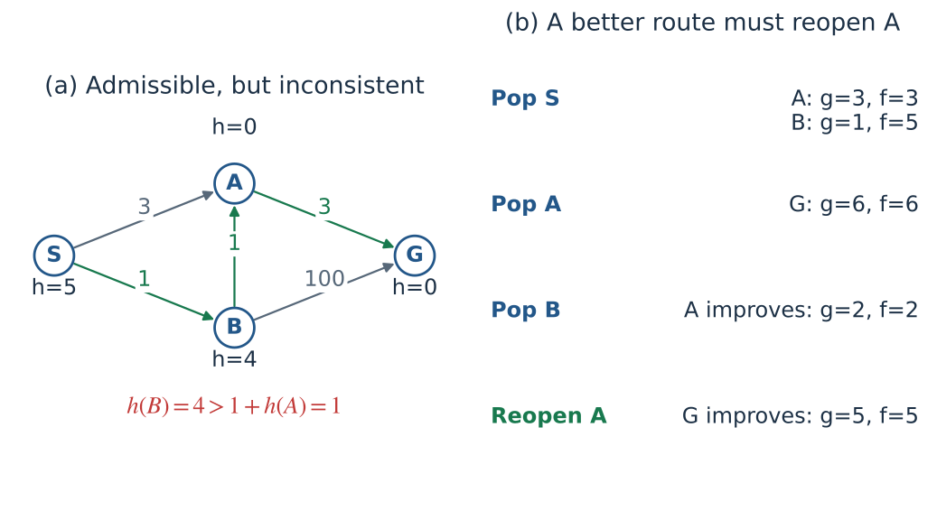
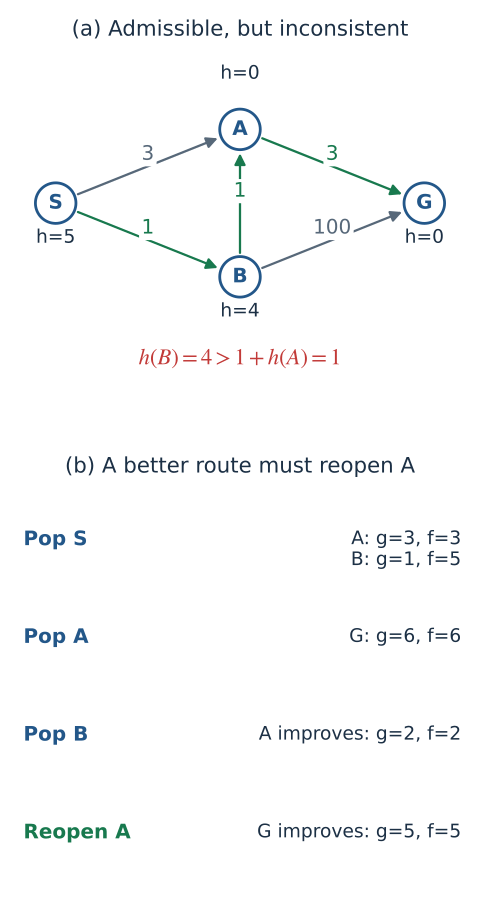
Figure 5. Admissibility alone does not justify a permanent closed set. The next implementation permits every strict cost improvement to reenter the queue.

9.2 Heuristic detective: catch the broken guarantee

Heuristic detective: catch the wrong answer

Controls

Loading interactive model…

Model & data

Finite directed graph: S→A=3, S→B=1, B→A=1, A→G=3, B→G=100. The exact remaining costs h* are (5,3,4,0) in S,A,B,G order; the optimum is S→B→A→G, cost 5. Presets: zero=(0,0,0,0), exact=(5,3,4,0), admissible but inconsistent=(5,0,4,0), overestimated=(0,0,8,0). Priorities are g+h, ties use lower h then insertion order, and the goal is accepted when popped. With reopening off, improvements to already expanded states are deliberately discarded: this is an incorrect general-A* variant used to expose the failure. With the inconsistent preset it returns cost 6; reopening restores cost 5. An overestimated h can return cost 6 even with reopening. Expanded excludes the goal. No result is stored or transmitted.

Choose the admissible-but-inconsistent preset and predict the next popped state before each step. Leave reopening enabled first, then disable it and replay the same graph. A is expanded at cost 3 before B improves it to 2. With reopening, the answer is 5; with permanent closing, it is 6. The graph and objective have not changed—only whether a better prefix is allowed to propagate.

Next choose the overestimated preset. It assigns B a remaining-cost estimate of 8 even though the true value is 4. A* can now accept the cost-6 goal before exploring B, even with reopening enabled. Reopening repairs the closed-set mistake; it does not repair a heuristic that overestimates.

Compare these runs with the exact-distance preset. Check admissibility state by state and consistency edge by edge. One bad local inequality disproves consistency. A successful answer on one run does not prove either condition.

A* as Dijkstra on reweighted edges

Define a new edge cost

\[\begin{aligned} c_h(u,v)&=c(u,v)\\ &\quad+h(v)-h(u). \end{aligned} \tag{15}\]

Consistency says exactly that $c_h(u,v)\ge0$. The heuristic terms telescope along a route from S to $n$:

\[\begin{aligned} g_h(n)&=g(n)+h(n)-h(s)\\ &=f(n)-h(s). \end{aligned} \tag{16}\]

Subtracting the same constant $h(s)$ from every priority does not change the ordering. Consistent A* therefore behaves like Dijkstra on these nonnegative reweighted edges. Every complete start-to-goal path changes by the same constant $h(t)-h(s)$, so the ordering of complete path costs is preserved too. This explains both the optimality and the no-reopening property without requiring A* to be memorized as a separate theorem.

10. A complete Python A* with lazy deletion and reopening

The function accepts a fixed heuristic(node) and a nonnegative weight. Ordinary A* uses weight=1; Dijkstra uses zero. The weighted variant is discussed separately below. Graphs use the same adjacency-list format as before.

import math

def astar(graph, start, goal, heuristic, weight=1.0):
    if not math.isfinite(weight) or weight < 0:
        raise ValueError("weight must be finite and nonnegative")

    # Cache a state-only heuristic: changing estimates during search would
    # invalidate this implementation's stored priorities and its proof.
    h_cache = {}
    def h(node):
        if node not in h_cache:
            value = float(heuristic(node))
            if not math.isfinite(value) or value < 0:
                raise ValueError("heuristic must be finite and nonnegative")
            h_cache[node] = value
        return h_cache[node]

    if h(goal) != 0:
        raise ValueError("the goal heuristic must be zero")
    serial = count()
    best_g = {start: 0.0}
    parent = {start: None}
    # Tuple fields: priority, h tie-breaker, unique serial, g snapshot, state.
    heap = [(weight * h(start), h(start), next(serial), 0.0, start)]
    expansion_order = []  # Includes repeated expansions after reopening.

    while heap:
        _priority, _h, _serial, g_entry, u = heappop(heap)
        if g_entry != best_g[u]:
            continue  # Skip an obsolete g snapshot before testing the goal.
        if u == goal:
            return reconstruct(parent, goal), g_entry, expansion_order

        expansion_order.append(u)
        for v, edge_cost in graph.get(u, []):
            if not math.isfinite(edge_cost) or edge_cost < 0:
                raise ValueError("edge costs must be finite and nonnegative")
            candidate = g_entry + edge_cost
            if not math.isfinite(candidate):
                raise OverflowError("path cost overflow")
            if candidate < best_g.get(v, math.inf):
                best_g[v] = candidate
                parent[v] = u
                # No closed-set rejection: even an expanded state may improve.
                heappush(heap, (candidate + weight * h(v), h(v),
                                next(serial), candidate, v))

    return None, math.inf, expansion_order

H = {"S": 3, "A": 1, "B": 2, "C": 1, "G": 0}
path, cost, expanded = astar(graph, "S", "G", H.__getitem__)
assert path == ["S", "B", "C", "G"] and cost == 5

reopen_graph = {
    "S": [("A", 3), ("B", 1)], "A": [("G", 3)],
    "B": [("A", 1), ("G", 100)], "G": [],
}
RH = {"S": 5, "A": 0, "B": 4, "G": 0}
path, cost, expanded = astar(reopen_graph, "S", "G", RH.__getitem__)
assert cost == 5 and expanded == ["S", "A", "B", "A"]

In the examples, H.__getitem__ passes the dictionary’s lookup operation as a function: calling it with a node returns H[node]. Writing lambda node: H[node] would do the same job. The graph stores legal moves and costs; the separate dictionary stores the heuristic chosen for this goal.

The returned expansion list excludes the goal, whose outgoing edges are not inspected. Some tools count that final removal as an expansion; either convention is usable, but comparisons need to state which one they use.

The loop follows the same relaxation pattern as Dijkstra. Read g_entry as a snapshot of the prefix price when that heap entry was inserted. If a better route has since changed best_g[u], the snapshot is stale and the loop skips it. Only after that check can the entry trigger the goal return or expand outgoing edges. For each neighbor, candidate is a real route price; a strict improvement updates both best_g and parent, then pushes a fresh entry. There is no permanent “already expanded, reject forever” test, so the same code handles reopening without a separate repair routine.

The heap stores five fields rather than a node alone because it must answer several different questions: which candidate has the smallest priority, how ties are resolved, which prefix price this entry represents, and which state should be expanded. Python compares tuples from left to right. count() supplies a different serial value on every insertion, so comparison is decided before it could reach arbitrary state objects. The fourth field is not another priority; it is the cost snapshot used by the stale-entry check.

The second heap field prefers smaller $h$ among equal priorities. Under ordinary A* this also prefers larger $g$ on an exact $f$ tie. The serial number makes the final choice deterministic and prevents Python from trying to compare arbitrary node objects. Changing tie-breaking can change the path or number of expansions without changing the optimal cost.

The stale check uses equality of the stored floating-point snapshot with the very value copied into best_g. It does not recompute a sum and compare two independent arithmetic expressions. Adding a large tolerance to the strict relaxation test can silently discard a genuinely better route. Integer costs avoid many numerical issues; with floating costs, test near ties explicitly.

The function checks that heuristic values are finite and nonnegative, and that the goal’s value is zero. It cannot establish admissibility from those checks; the lower-bound argument remains the caller’s responsibility. It also validates only edges it encounters, not an entire implicit graph in advance.

11. Grid heuristics must match the movement rules

The search loop does not require coordinates, but a grid gives us a cheap way to calculate the remaining-cost estimate. The current state has coordinates (x, y) and the target has coordinates (x_t, y_t). Only their separation matters for the wall-free calculation. Write

\[\begin{aligned} \Delta x&=\lvert x-x_t\rvert,\\ \Delta y&=\lvert y-y_t\rvert,\\ m&=\min(\Delta x,\Delta y),\\ M&=\max(\Delta x,\Delta y). \end{aligned}\]

The absolute values make both separations nonnegative, regardless of which direction the target lies. For a move from (0, 0) to (3, 2), the horizontal and vertical separations are 3 and 2; m=2 is the smaller separation and M=3 the larger. The symbols $D$ and $D_2$ below are costs per move, not coordinate distances: $D$ is an orthogonal-step lower bound and $D_2$ a diagonal-step lower bound.

11.1 Four directions

If every orthogonal move costs at least $D$, Manhattan distance is

\[h_4=D(\Delta x+\Delta y). \tag{17}\]

For that (3, 2) displacement and unit-cost moves, three horizontal corrections and two vertical corrections require at least five moves. Their order can change, but their total cannot fall below five. A wall might force seven moves instead; the heuristic remains five because it deliberately ignores that extra restriction.

Euclidean distance,

\[h_E=D\sqrt{\Delta x^2+\Delta y^2}, \tag{18}\]

is also a lower bound here, but usually weaker. Its being a familiar geometric distance does not automatically make it the best heuristic for a grid.

For the same displacement, Euclidean distance is about 3.61 while Manhattan distance is 5. “Weaker” means that it leaves more of the unavoidable cost unaccounted for, not that it is mathematically invalid. The character cannot realize that straight-line movement when only horizontal and vertical steps are legal.

11.2 Eight directions

Suppose an orthogonal move costs at least $D$ and a diagonal costs at least $D_2$, with

\[D\le D_2\le2D.\]

In the obstacle-free relaxed grid, take $m$ diagonals to reduce both coordinate differences, then $M-m$ orthogonal steps:

\[\begin{aligned} h_8&=D_2m+D(M-m)\\ &=D(\Delta x+\Delta y)\\ &\quad+(D_2-2D)m. \end{aligned} \tag{19}\]

For $D_2=\sqrt2D$, this is octile distance. If diagonals and orthogonal steps both cost $D$, it becomes Chebyshev distance, $D\max(\Delta x,\Delta y)$.

For (0, 0) → (3, 2), two diagonals remove two units from both separations, leaving one horizontal step. With unit orthogonal cost and diagonal cost about 1.414, the relaxed route costs about 3.83. If diagonals cost one instead, those same three moves cost 3. The heuristic changes because the allowed actions became cheaper, not because the goal moved.

The assumed cost range explains this construction. A diagonal costs no more than the two orthogonal steps it replaces, but no less than one orthogonal step. Taking a pair of diagonals in a zigzag therefore cannot make progress along a single axis cheaper than ordinary straight steps. Outside this range, the cheapest relaxed route needs a different argument.

Manhattan distance is generally not admissible when a diagonal costs $\sqrt2D$: from $(0,0)$ to $(1,1)$, it estimates $2D$ even though a single diagonal costs $\sqrt2D$. A small change in movement rules changes the proof.

For the diagonal-$\sqrt2$ model, Euclidean distance remains admissible because every move costs at least $D$ times its Euclidean length. If diagonals cost only $D$, that particular Euclidean scaling can overestimate; Chebyshev is the appropriate relaxed distance.

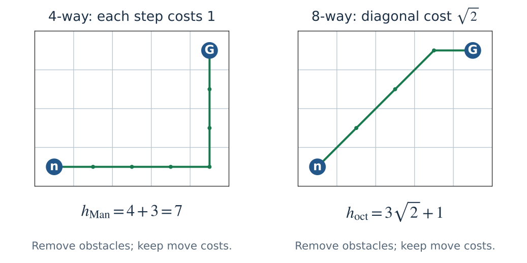
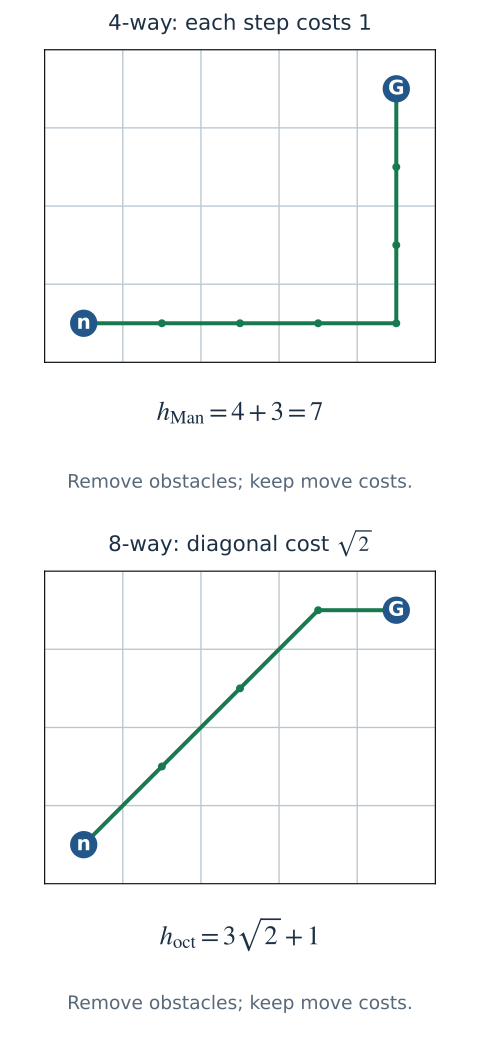
Figure 6. A heuristic is tied to legal moves and their minimum costs. Removing walls may lower the optimum; permitting cheaper diagonal moves can invalidate a four-way estimate.

11.3 Terrain costs and units

The editable labs use a destination-entry multiplier $q(v)$:

\[\begin{gathered} c(u,v)=\ell(u,v)\,q(v),\\ q(v)\in\{1,5\},\\ \ell(u,v)\in\{1,\sqrt2\}. \end{gathered} \tag{20}\]

The start tile costs nothing until a move enters another tile. Because $q(v)$ belongs to the destination, traversing the same geometric edge backward may have a different cost. That is a directed weighted graph even though movement is allowed both ways.

For example, an orthogonal move from grass into mud costs 5; returning from that mud tile into grass costs 1. The terrain label is not a fee for standing on a tile, and both ends are not charged. This convention turns the visible terrain into the exact edge costs used by relaxation.

Multiply the geometric heuristic by a global lower bound $q_{\min}$ on traversable terrain costs, not the average terrain cost or the current tile’s multiplier. Here $q_{\min}=1$. If some terrain costs 0.2, a unit-scaled Manhattan heuristic may overestimate; using $q_{\min}=0.2$ restores the lower bound. With zero-cost terrain and no stronger argument, $h=0$ is safe.

Units must agree. If $g$ is measured in seconds, $h$ must be a lower bound in seconds, such as straight-line distance divided by a valid upper bound on speed. Adding meters to seconds does not become meaningful because both are floating-point numbers.

The labs forbid corner cutting: a diagonal is legal only when both adjacent orthogonal cells are free. Ignoring that restriction when computing a heuristic merely relaxes the problem and remains safe; ignoring it when generating actual neighbors permits illegal paths.

Generate the grid edges in Python

rows[y][x] selects a row first, then a column. Each (dx, dy) is a proposed one-step displacement; free rejects a destination outside the map or inside a wall. math.hypot(dx, dy) calculates the step’s geometric length: 1 for an orthogonal move and about 1.414 for a diagonal. The function combines that length with the destination terrain and returns the same adjacency-list format used by astar.

def grid_graph(rows, diagonal=False):
    # '#' is blocked; '.'/'S'/'G' cost 1 to enter; '5' costs 5.
    height, width = len(rows), len(rows[0])
    if any(len(row) != width for row in rows):
        raise ValueError("rows must have equal length")
    moves = [(1, 0), (0, 1), (-1, 0), (0, -1)]  # E, S, W, N
    if diagonal:
        moves += [(1, 1), (-1, 1), (-1, -1), (1, -1)]
    def free(x, y):
        return 0 <= x < width and 0 <= y < height and rows[y][x] != "#"
    result = {}
    for y in range(height):
        for x in range(width):
            if not free(x, y):
                continue
            edges = []
            for dx, dy in moves:
                nx, ny = x + dx, y + dy
                if not free(nx, ny):
                    continue
                if dx and dy and not (free(x + dx, y) and free(x, y + dy)):
                    continue  # Both sides of a diagonal must be clear.
                terrain = 5 if rows[ny][nx] == "5" else 1
                edges.append(((nx, ny), math.hypot(dx, dy) * terrain))
            result[(x, y)] = edges
    return result

rows = [".......", ".S555G.", "......."]
grid = grid_graph(rows)
start, goal = (1, 1), (5, 1)
manhattan = lambda n: abs(n[0] - goal[0]) + abs(n[1] - goal[1])
path, cost, _ = astar(grid, start, goal, manhattan)
assert cost == 6  # Six grass steps beat entering three mud tiles (cost 16).
assert len(bfs(grid, start, goal)) - 1 == 4

On the middle row, going straight from S to G uses four moves: enter three mud tiles, then G, for cost 5 + 5 + 5 + 1 = 16. Going up once, across four grass tiles, then down to G uses six moves but costs only 6. That is why the BFS assertion checks four moves, while the A* assertion checks a cost of 6. The lambda n supplies a function that reads the coordinate pair as n[0] and n[1]; it is the Manhattan formula written directly in Python.

Weighted routes: compare the priorities

Controls

Loading interactive model…

Model & data

Directed edge cost c(u,v)=step length×terrain(v); terrain is 1 or 5, and the start has no entry charge. Orthogonal steps cost length 1; diagonals length √2. Diagonals require both adjacent orthogonal cells to be open. Heuristics use the minimum terrain multiplier 1. Manhattan is restricted to four-direction movement; Euclidean and octile are safe for eight. A* uses g+w h, with reopening on every strict g improvement and stale-entry rejection. Ties use lower h then insertion order. Reference cost is freshly computed by Dijkstra on the same edited grid. Expanded counts successor expansions, including repeat expansions after reopening, but excluding the goal. Frontier and peak count distinct active states, not raw heap entries; obsolete heap entries are excluded.

Compare BFS, Dijkstra, greedy, and A* on the same map. First keep four-direction movement and heuristic weight one. Paint a few mud tiles on the direct route, then move a wall to create a detour. Watch path cost, expanded states, and the Dijkstra reference separately. A search that removes fewer candidates is not better if it solves a different objective.

Switch to eight directions and inspect the heuristic selection. The lab restricts the available lower bounds to those compatible with its movement costs. Use the edit mode and click a cell, or focus the map and use the arrow keys and the indicated keyboard action. Editing the map starts a new search rather than changing the graph underneath an old frontier.

11.4 Sliding tiles: A* on a graph you cannot draw all at once

Move a numbered tile into the adjacent blank until the board reads 1 through 8, with the blank last. A state is all nine entries in row-major order; an edge swaps the blank with one neighboring tile. Every swap costs one. The board’s nine visible squares are not the nine graph states—the whole arrangement is one state.

“Row-major” means reading the top row left to right, then the middle row, then the bottom row. For example, (1, 2, 3, 4, 5, 6, 7, 0, 8) uses 0 for the blank. Moving tile 8 left produces the goal arrangement. Both the old and new arrangements are single vertices; the swap is the edge between them. Since every edge costs one, BFS would also find a shortest solution. A* uses the tile estimate to prioritize promising arrangements instead of processing the entire distance layer indiscriminately.

The 8-puzzle: play first, then race A*

Controls

Loading interactive model…

Model & data

A state is a row-major permutation of tiles 1–8 and blank 0. A legal move swaps the blank with an orthogonally adjacent tile and costs 1. Goal: 123456780. Presets have exact optimal distances 4, 8 and 12, verified by reverse BFS—not by counting scramble moves. Manhattan h sums numbered-tile distances and excludes the blank. The h=0 setting is Dijkstra. Ties use lower h, then insertion order; neighbor order moves the blank right/down/left/up. Goal acceptance is on a valid minimum-priority pop. Expanded excludes the goal. The solver rejects stale entries and reopens on strict g improvements; a run stops after at most 50,000 valid pops. Finish runs in scheduled batches. Manual play and solver playback are separate. All state stays in the browser; no score is stored or sent.

Play a few moves yourself, then compare the solver with Manhattan guidance and with zero heuristic. The presets have optimal distances 4, 8, and 12, verified by reverse BFS from the goal. These numbers are not merely the number of random shuffling moves: a shuffle can undo itself or revisit an earlier arrangement.

For each numbered tile, count its horizontal and vertical displacement from its goal square, then sum. Here x and y are column and row indices, and the superscript “goal” marks the target coordinates:

\[\begin{aligned} h_{\mathrm{tiles}}(s) &=\sum_{k=1}^{8}\bigl(\lvert x_k-x_k^{\mathrm{goal}}\rvert\\ &\qquad+\lvert y_k-y_k^{\mathrm{goal}}\rvert\bigr). \end{aligned}\]

Exclude the blank. A legal move changes the position of exactly one numbered tile by one square, so it can reduce this sum by at most one. Reducing the sum to zero therefore needs at least that many moves: the heuristic is admissible. The same one-step bound also gives consistency.

Compute the tile heuristic and test why the blank is excluded

def tile_manhattan(board):
    total = 0
    for index, tile in enumerate(board):
        if tile == 0:
            continue  # Blank is an action mechanism, not another goal tile.
        y, x = divmod(index, 3)
        goal_y, goal_x = divmod(tile - 1, 3)
        total += abs(x - goal_x) + abs(y - goal_y)
    return total

assert tile_manhattan((1, 2, 3, 4, 5, 6, 7, 8, 0)) == 0
assert tile_manhattan((1, 2, 3, 4, 5, 6, 7, 0, 8)) == 1
assert tile_manhattan(tuple(map(int, "123687540"))) == 10

divmod(index, 3) returns the quotient and remainder, which are the row and column of a position in a three-column board. tile - 1 converts a numbered tile into its goal’s zero-based position. In the one-move-away board, tile 8 is at index 8, or row 2/column 2, but belongs at index 7, or row 2/column 1. Its contribution is one; every other numbered tile contributes zero.

In the one-move-away board, counting both tile 8 and the blank would give 2 although the real remaining cost is 1. In the depth-12 preset, the numbered-tile estimate is 10: interactions among tiles require work that the relaxed sum does not count. That is an underestimate, not a bug.

12. What A* saves—and what it cannot promise

12.1 The optimal-cost boundary

Suppose the optimal route costs 16. A candidate with recorded prefix cost 7 and remaining lower bound 4 has priority 11. It might still lead to a route cheaper than 16, so the lower bound does not rule it out. It does not assert that an 11-cost complete route exists. A candidate with prefix cost 12 and lower bound 6 has priority 18; it can wait while a goal costing 16 is available. A* does not know the optimal cost 16 in advance: the optimal-prefix frontier argument explains why the cheaper possibility stays ahead of an expensive goal.

Before an optimal goal is removed, an admissible A* frontier contains an optimal-prefix entry with $f\le C^{\ast}$. Thus it does not need to select a candidate with $f>C^{\ast}$ before returning an optimal answer. Under a consistent heuristic, reachable states with $g^{\ast}(n)+h(n)<C^{\ast}$ are expanded; states on the equality boundary depend on tie-breaking and when the goal is removed.

The optimal prefix cost in this inequality is a theoretical value, not necessarily the current best_g entry. The code compares current priorities with one another; it does not receive the unknown optimal cost as a pruning threshold. The boundary explains which work the priority ordering can avoid.

Increasing a lower bound can shrink the region strictly below this boundary. If two admissible heuristics satisfy $h_2(n)\ge h_1(n)$ for every state, $h_2$ dominates $h_1$. But “larger heuristic means fewer operations on every run” is too strong: equal-priority plateaus, reopening, heuristic evaluation cost, and tie-breaking still matter.

Even an exact $h=h^{\ast}$ need not produce one expansion per path step. Many states can lie on equally good routes and have $f=C^{\ast}$. Favoring smaller $h$ on ties often helps reach a goal through that plateau; it does not improve the optimal cost.

12.2 Complexity depends on the implementation and the state space

There are several different kinds of work. Expansions count states whose successors are examined. One expansion may inspect many edges, generate several heap entries, and call the heuristic for previously unseen states. Elapsed time includes all of these operations. Peak memory measures what must be retained simultaneously. Fewer expansions need not mean less time if each heuristic evaluation is expensive.

The following operation-count bound assumes constant-time edge-cost access, average constant-time dictionary operations, and constant-time heuristic evaluation. A cached but expensive heuristic still has to be computed once for each newly encountered state. Here $T$ denotes time complexity and $M$ auxiliary memory; the reuse of $M$ does not refer to the larger coordinate separation defined in Section 11.

For Dijkstra or consistent A* on a finite explicit graph, each state is validly expanded at most once. A lazy binary-heap implementation can hold $O(\lvert E\rvert)$ entries because improvements add duplicates. A conservative bound is

\[\begin{aligned} T&=O\bigl(\lvert V\rvert\\ &\qquad+\lvert E\rvert\log(2+\lvert E\rvert)\bigr),\\ M&=O(\lvert V\rvert+\lvert E\rvert). \end{aligned} \tag{21}\]

including cost/parent maps and the lazy heap, but not counting the input graph twice. Each examined edge can create a cheaper entry, and each heap insertion or removal has a logarithmic cost in the heap size. That accounts for the edge-count term multiplied by a logarithm. For an implicit puzzle, “number of states” means distinct complete arrangements, not the nine positions on one board.

Why a different heap gives a different bound

An indexed heap with a decrease-key operation keeps one live heap record per state and gives the familiar $O((\lvert V\rvert+\lvert E\rvert)\log(2+\lvert V\rvert))$ time and $O(\lvert V\rvert)$ auxiliary-space bound. It updates an entry in place instead of leaving an obsolete one behind. The Python implementation uses the simpler lazy strategy, so its heap can contain more records than there are distinct frontier states.

With an inconsistent heuristic, reopenings can make A* inspect edges repeatedly, so the once-per-state bound no longer applies. With an implicit search tree, the number of distinct states can itself be exponential in solution depth. A* is not a polynomial-time solution to arbitrary planning problems.

In practice, A* can use much more memory than DFS: it retains a frontier and best-known costs for many competing states. It can also lose to Dijkstra when the heuristic is expensive and provides little discrimination.

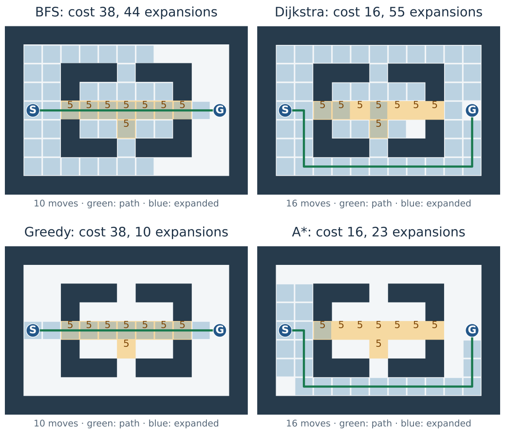
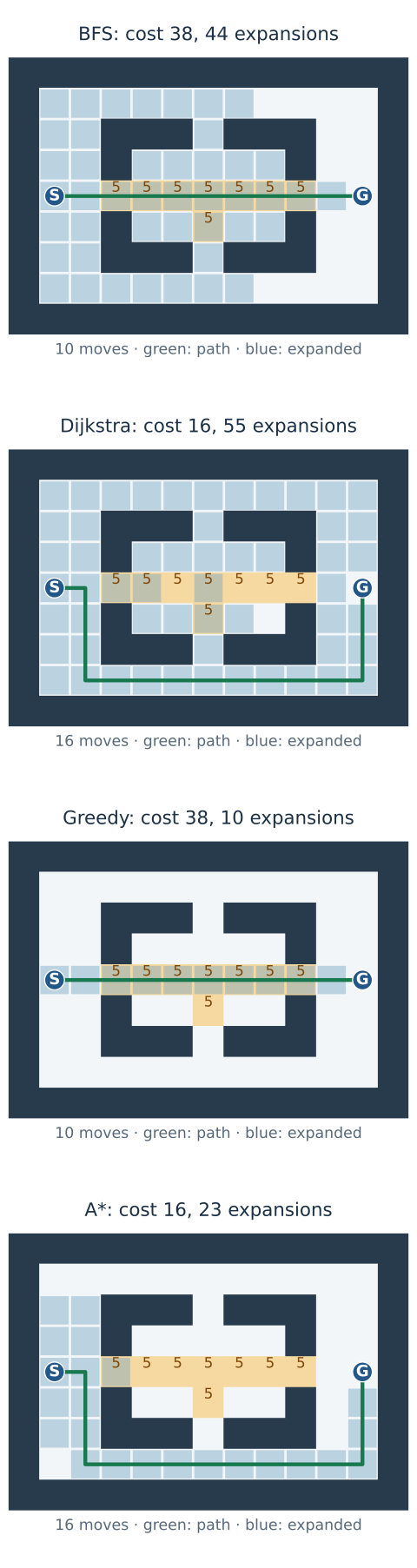
Figure 7. The fixed map, terrain costs, neighbor order, and tie policy are shared by the plotted searches. Cost and search effort are distinct outputs. These are counts for this map, not a universal speed ranking.

Search on Figure 7’s map	Returned cost	Moves in returned path	Expansions, excluding the goal
BFS	38	10	44
Dijkstra	16	16	55
Greedy	38	10	10
A*	16	16	23

Read across a row before comparing algorithms. BFS’s ten moves are cheap in step count, not in terrain cost: seven mud entries and three ordinary entries cost 7 × 5 + 3 = 38. Dijkstra and A* instead return sixteen unit-cost entries. Their answer quality is the same here; the difference is the 55 versus 23 expansions needed to find it. Greedy’s ten expansions look attractive only until its returned cost of 38 is considered.

Select Figure 7 comparison maze in the editable lab to reproduce this map. The simpler Expensive direct road preset has fewer obstacles and a different optimal cost. In both presets, one grass entry costs 1 and one mud entry costs 5.

The exact map and Python reproduction

comparison_rows = [
    "#############",
    "#...........#",
    "#..###.###..#",
    "#..#.....#..#",
    "#S.5555555.G#",
    "#..#..5..#..#",
    "#..###.###..#",
    "#...........#",
    "#############",
]
comparison_grid = grid_graph(comparison_rows)
cs, ct = (1, 4), (11, 4)  # Zero-based x, y; y increases downward.
ch = lambda n: abs(n[0] - ct[0]) + abs(n[1] - ct[1])
cp, cc, ce = astar(comparison_grid, cs, ct, ch)
assert cc == 16 and len(cp) - 1 == 16 and len(ce) == 23
assert path_cost(comparison_grid, bfs(comparison_grid, cs, ct)) == 38

Neighbors are generated east, south, west, north. Heap searches break equal primary priorities by smaller Manhattan $h$, then insertion order. The short Dijkstra snippet above instead uses insertion order alone on a $g$ tie, so its expansion count can differ even though its optimal cost is the same. For the figure’s Dijkstra ordering, use astar(comparison_grid, cs, ct, ch, weight=0); the second tuple field still breaks ties by $h$.

12.3 A practical comparison

Method	Next candidate	Minimum-cost guarantee in the stated finite graph model	Typical reason to choose it
Graph DFS	Newest candidate	No	Reachability, structural traversal, low implementation overhead
Graph BFS	Oldest candidate	Equal-cost edges	Fewest moves in an unweighted problem
Exhaustive simple paths	Every candidate path	Yes, nonnegative costs	Tiny independent reference cases
Dijkstra / UCS	Smallest $g$	Nonnegative costs	No useful heuristic; distances to many goals
Greedy best-first	Smallest $h$	No	Fast candidate route when quality can be checked separately
A* with reopening	Smallest $g+h$	Admissible $h$	One goal and a useful remaining-cost lower bound

All of these finite graph searches can report failure if implemented with the appropriate duplicate handling. Greedy’s lack of optimality should not be confused with inevitable nontermination on a finite graph. The common warning that greedy can be incomplete concerns unrestricted infinite spaces or implementations that mishandle cycles.

13. Weighted A*: spend some optimality to prioritize the goal

Two meanings of “weighted” must be separated:

• A weighted graph has costs on edges. Ordinary A* already handles this.
• Weighted A* changes the priority to emphasize the heuristic:

\[f_w(n)=g(n)+w\,h(n). \tag{22}\]

The weight changes which candidate is processed next, not what the roads cost. Consider two hypothetical frontier entries. The last two columns compare ordinary A* with $w=2$:

Candidate	$g$	$h$	$g+h$	$g+2h$
X	2	5	7	12
Y	6	2	8	10

Ordinary A* selects X; weight 2 selects Y, which has the smaller remaining estimate despite its more expensive prefix. The returned route is still evaluated by adding the original edge costs. The inflated priority is a search preference, not a replacement objective.

At $w=0$ the primary priority is Dijkstra’s; at $w=1$ it is ordinary A*. For $0<w<1$, a nonnegative admissible heuristic remains admissible after scaling, so reopening A* remains optimal. For $w>1$, $wh$ may overestimate and the exact optimality proof no longer holds.

However, on a finite nonnegative-cost graph, with an admissible nonnegative base $h$, $h(t)=0$, a fixed $w\ge1$, reopening on every strict improvement, and stopping at valid goal removal, the returned cost satisfies

\[C_{\mathrm{returned}}\le w\,C^{\ast}. \tag{23}\]

For example, $w=1.5$ guarantees at most 1.5 times the optimal cost under those conditions. It does not mean the route will be 50% worse, or that runtime will fall by any particular factor. Increasing $w$ is not guaranteed to monotonically reduce expansions or monotonically increase path cost on every map.

If the true optimum is 16, that factor permits a returned cost up to 24. Returning 16 is still possible; the bound is a ceiling, not a target. The original admissible heuristic is the ingredient that justifies the ceiling even though its inflated version may no longer be admissible.

Derive the weighted bound

As in the ordinary A* proof, an unfinished optimal route has an optimal-prefix frontier entry $n$. For $w\ge1$,

\[\begin{aligned} f_w(n)&=g^{\ast}(n)+w h(n)\\ &\le g^{\ast}(n)+w h^{\ast}(n)\\ &\le w\bigl(g^{\ast}(n)+h^{\ast}(n)\bigr)\\ &=wC^{\ast}. \end{aligned} \tag{24}\]

The second inequality uses $g^{\ast}(n)\ge0$. When a valid goal is removed, its priority is exactly its path cost and cannot exceed this remaining frontier entry. The proof relies on retaining the optimal-prefix entry through reopening; it is not a license to combine arbitrary pruning rules with a weighted priority. Likhachev, Gordon, and Thrun’s ARA* paper develops bounded-suboptimal and anytime heuristic search further.

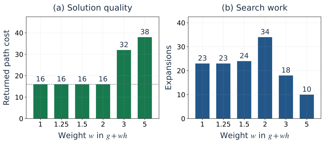
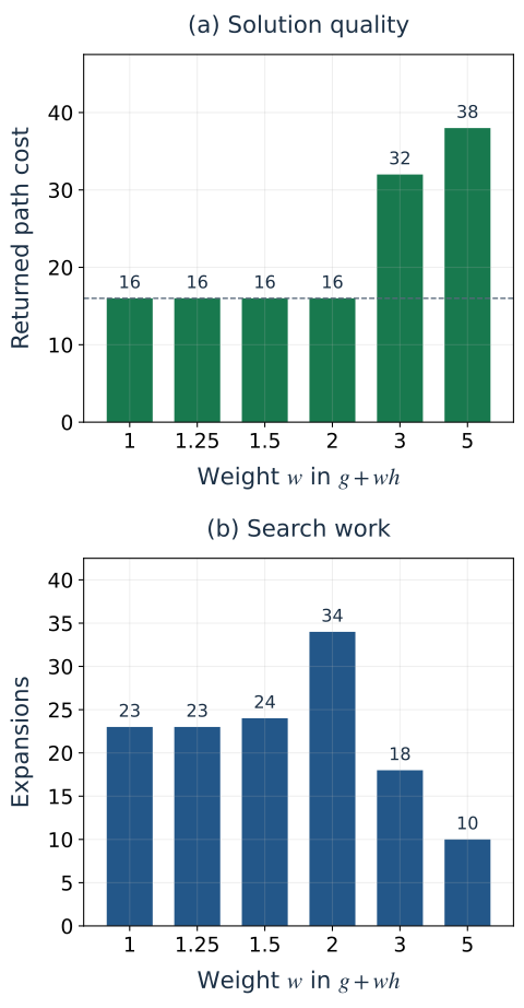
Figure 8. Each weight starts a fresh search on the same map. The $wC^{\ast}$ ceiling is a theorem under the stated assumptions, not a prediction of the actual returned cost.

13.1 Write a priority rule and test it

Write a priority expression

Controls

Loading interactive model…

Model & data

Restricted arithmetic editor, not a Python or JavaScript interpreter. Grammar: g, h, finite numbers, + - * / and parentheses; unary + and - are accepted. No functions, assignment, property access, loops or external code. At most 80 characters, 80 tokens and 16 nesting levels. Each run is bounded to 10,000 valid pops. Three authored four-direction test grids compare returned costs with Dijkstra. Passing these examples does not prove admissibility, consistency, completeness or optimality in general.

Enter g + h, run the test maps, then compare g, h, and g + 2*h. The editor accepts a restricted arithmetic expression in g and h; it is not an arbitrary JavaScript or Python runtime. This keeps a typo from executing unrelated code or an infinite loop. The downloadable notebook supports ordinary Python experiments.

A passing collection of test maps does not prove admissibility or a worst-case bound. The tests answer “what happened on these inputs?” The inequalities above answer “what must happen on every input satisfying the assumptions?” Both kinds of evidence are useful, but they are not interchangeable.

Try to explain each result before looking at the reference cost. Which expression ignores the price already paid? Which sacrifices exact optimality? Why might two expressions return the same route even though their guarantees differ?

14. Building and checking stronger heuristics

14.1 Combine lower bounds safely

If $h_1$ and $h_2$ are admissible, then

\[h(n)=\max\{h_1(n),h_2(n)\} \tag{25}\]

is admissible and at least as informative as either one: both estimates are no greater than the true remaining cost, so their maximum cannot exceed it either. If both are consistent, their maximum is consistent too. Choose whichever estimate supplies the maximum at $u$. Its consistency bounds it by $c(u,v)$ plus its own value at $v$. That value at $v$ cannot exceed the maximum there, so adding the same edge cost preserves the inequality.

Their sum is not generally admissible. Two estimates may count the same unavoidable movement twice. Adding separately admissible estimates needs a cost-partitioning or disjoint-subproblem argument, not merely two successful tests.

For the one-move-away tile puzzle, imagine two methods that both give the valid lower bound one. Taking their maximum still gives one. Adding them gives two, which is already larger than the actual one-move solution. Each method can be correct on its own while their sum is wrong, because they counted the same required move.

14.2 Exact distances are a useful testing oracle

On a finite graph, compute $h^{\ast}(n)$ by running Dijkstra from the goal on the reversed graph. Reversing an edge $u\to v$ keeps the original numeric cost $c(u,v)$ on the new edge $v\to u$. With destination-entry terrain, recomputing the cost from the new destination would change the problem.

This is a way to calculate all the remaining distances in one run. In the original five-state example, the route S → B → C → G costs 3 + 1 + 1 = 5. Its reversed counterpart G → C → B → S costs 1 + 1 + 3 = 5. Every original route to G corresponds to a reversed route from G with the same cost. Ordinary forward search from G would not work: G has no outgoing edges in the original graph. Reversal is bookkeeping for the original journey, not permission to travel backward along an originally one-way road.

An offline checker can then test

\[\begin{gathered} h(n)\le h^{\ast}(n),\\ h(u)\le c(u,v)+h(v). \end{gathered} \tag{26}\]

for every state and edge. This can establish the properties on that particular fully enumerated graph. It does not prove that a formula works for every map size or cost model.

Computing exact goal distances before one A* query may cost as much as solving the original problem. It becomes worthwhile when many starts share the same static goal, or when those distances support a broader preprocessing scheme.

Landmark lower bounds on undirected graphs

For a landmark $L$ in an undirected nonnegative-cost graph, the triangle inequality gives

\[\begin{aligned} h_L(n)&=\left\lvert d(L,t)-d(L,n)\right\rvert\\ &\le d(n,t). \end{aligned} \tag{27}\]

Here $d$ denotes minimum path cost between its two arguments, not necessarily geometric distance. Use landmarks for which the required distances are finite, for example within the goal’s connected component; otherwise skip that landmark. Subtracting two infinite distances would be undefined. If no landmark supplies a usable bound, zero remains safe.

Take the maximum across several landmarks to strengthen the bound. Distances to landmarks can be precomputed once for a static graph. For directed graphs the absolute-value formula is not generally valid. Where the needed distances are finite, valid directed bounds instead include $d(L,t)-d(L,n)$ and $d(n,L)-d(t,L)$, together with zero. The ALT work by Goldberg and Harrelson combines A*, landmarks, and triangle inequalities for route planning.

15. Modeling errors that no priority rule can repair

An incomplete state. If two arrivals at a tile have different fuel, keys, orientation, or arrival times and those affect the future, position alone is not a valid state. A smaller $g$ at the same coordinate may not dominate a more expensive arrival with more remaining fuel. Include the relevant variables in the state or use a suitable multi-label method.

An objective that is not the desired one. Minimizing distance does not automatically minimize time, risk, energy, or turning effort. Costs can combine penalties, but the units and tradeoff coefficients must have a defined meaning. A* optimizes the supplied scalar sum, not a human’s unstated preference.

Changing costs mid-search. The proof assumes one fixed graph. If a door closes or terrain cost changes, simply continuing with stale costs and parents can produce invalid results. Restart for a small problem, or use an incremental planning method designed to repair earlier results.

An optimistic collision model. A point moving between tile centers is not a robot with width and turning radius. Inflate obstacles by the required clearance, check transitions for collision, or use a richer configuration-space model. A valid graph route may still require continuous trajectory planning.

A heuristic that ignores a shortcut incorrectly. Ignoring walls is safe because it makes the problem easier. Ignoring an available teleport while retaining ordinary distance can make the estimate too large, because the real problem may now be cheaper than the imagined wall-free walk.

Unfair benchmarks. Compare the same start, goal, obstacles, cost model, movement rules, tie policy, and stopping rule. Count expansions, generated entries, peak frontier size, path cost, and elapsed time separately. Browser animation time is not algorithm runtime; one step may deliberately wait so that a person can see it.

16. Where A* is useful, and where another method fits better

Games and navigation meshes

Grid cells, polygon regions, or waypoint intersections can serve as states. A* is useful when the destination is known and a cheap geometric lower bound is informative. The resulting route still needs movement control and collision handling. For many units moving toward one fixed goal, a reverse shortest-path tree or flow field can be more economical than separate A* searches.

The mapping is concrete: a waypoint is a state, a traversable connection is an edge, its traversal time is a possible cost, and the destination waypoint is the goal. A navigation mesh represents walkable space with connected polygons rather than individual square tiles. A shared flow field tells units which next connection leads toward the common destination, using the precomputed remaining costs.

Grid-specific extension: Jump Point Search

Jump Point Search prunes symmetric grid exploration under specific uniform-cost movement assumptions. It is not a drop-in pruning rule for arbitrary terrain weights. Harabor and Grastien’s original paper states the grid setting and pruning rules.

Robotics and dynamic maps

For a robot that cannot move sideways, (x, y, heading) can be a more useful state than position alone. A short forward movement or a permitted turn creates an edge; its duration or energy is the edge cost. A motion primitive is one such predefined short movement. Checking collisions decides which edges exist; it is a separate job from deciding their search priority.

The endpoint position and orientation after each primitive define a state in the robot’s discrete configuration space: the set of configurations represented by the model. A* searches these states, while a heuristic comes from a simpler obstacle-free or lower-dimensional problem. D* Lite reuses information as relevant edge costs change rather than solving every update entirely from scratch; see Koenig and Likhachev.

Any-angle extension: Theta*

Theta* permits line-of-sight parent connections to produce any-angle routes on grids. Its graph and relaxation rules differ from ordinary grid A*, and it is not guaranteed to find the true continuous shortest path in general. Daniel and colleagues give the algorithm and its limitations.

Road routing and large static graphs

Straight-line distance divided by a genuine maximum speed is a possible travel-time lower bound, but preprocessing can be much more powerful for repeated queries. Landmark methods such as ALT strengthen A*; hierarchical methods and contraction-based routing can also exploit road-network structure. A* is one component of route planning, not an accurate description of every production map service.

Puzzles and symbolic planning

For a sliding-tile puzzle, a state is an entire tile arrangement and a move swaps the blank with a neighbor. With one moved tile per unit-cost action, summing each tile’s Manhattan distance to its target, excluding the blank, is admissible: a move changes one tile’s distance by at most one. Stronger pattern databases store exact distances for relaxed subproblems. Adding pattern values needs a valid disjoint-cost construction.

The same structure appears in planning: a state describes facts, an edge is an action, and the cost measures the objective. The hardest work is often designing a compact state and a strong lower bound, not implementing the heap.

For example, (room, have_key, door_open) can describe a tiny planning problem. Picking up a key, unlocking a door, and entering the next room are actions with preconditions and effects. If every action costs one and the goal is to reach a particular room, search minimizes action count. It is the same frontier mechanism used for the water jugs, but with different successor rules.

Memory limits and anytime answers

Ordinary A* keeps many alternatives so that it can compare them later. When that storage is the limiting resource, a different algorithm must decide what information to discard or recompute. An anytime method instead addresses a time budget: it can provide a feasible answer first and improve that answer while more computation is allowed.

Memory-conscious and anytime variants: IDA* and ARA*

IDA* performs repeated depth-first searches bounded by an $f$ threshold, trading repeated work for much lower memory in common tree-search formulations. ARA* starts with an inflated heuristic and refines solution quality while reusing search work. These methods solve different resource constraints; neither implies that ordinary A* will fit in memory on a huge state space.

Reasons not to choose A*

Use BFS when all edge costs are equal and the graph is modest. Use Dijkstra when no useful heuristic exists or many destinations need distances from one start. On a directed acyclic graph, a topological-order shortest-path algorithm can be simpler and supports negative edges. For general negative edges use a suitable algorithm such as Bellman–Ford, with negative-cycle handling. If multiple agents must avoid one another, independent single-agent A* routes do not solve their joint coordination problem.

17. Questions worth answering before calling an implementation correct

17.1 Five problems, five pictures

Each problem gives a graph or a movement model. Choose an answer from that input, then compare your reasoning with the explanation. The five problems test goal acceptance, reopening, movement costs, boundary cases, and geometric lower bounds. Hints and your previous answers remain available as you move between problems.

Five illustrated A* exercises

Controls

Loading interactive model…

Model & data

Five finite illustrated problems cover goal acceptance, reopening, move-dependent distance, boundary cases and a speed-based heuristic. Arrow labels are directed edge costs unless stated otherwise. Answers and hints remain only in this page session; Reset clears them. Diagrams and bilingual explanations come from one local JSON source shared with the notebooks.

17.2 Coding test: complete the A* core

Task. Complete astar_cost(graph, start, goal, h). The input is a finite directed graph with nonnegative edge costs and a supplied nonnegative admissible heuristic, with h[goal] == 0. Return the minimum path cost, or None if no route exists. When start equals goal, return 0. The heuristic need not be consistent, so a cheaper route must be allowed to update an already expanded state.

The search scaffold already supplies the heap, cost snapshots, stale-entry rejection and reinsertion. Complete three decisions: the priority expression using g and h, the relaxation condition using candidate and old_g, and the point at which the goal is accepted. The heap breaks ties by smaller h, then insertion order. Expansion counts exclude the goal.

In the illustrated example, A looks closest because its heuristic is zero, but the final edge from A is expensive:

exercise_graph = {
    "S": [("A", 1), ("B", 4)],
    "A": [("G", 20)],
    "B": [("G", 1)],
    "G": [],
}
exercise_h = {"S": 5, "A": 0, "B": 1, "G": 0}

# Expected output for astar_cost: 5, from S -> B -> G.
# Check the same input with the complete search from section 10.
assert astar(exercise_graph, "S", "G", exercise_h.__getitem__)[1] == 5

The judge checks both returned costs and two explicit expansion budgets. In particular, the open 15×15 grid permits at most 40 expansions. With the stated tie rule, ordinary A* expands 28 states and Dijkstra expands 224. Dijkstra still returns the correct cost; this case checks whether the supplied heuristic actually saves work. These counts belong to this test grid, not a general speed guarantee.

Coding test: complete the three A* decisions

Controls

Loading interactive model…

Model & data

Guided coding test, not an arbitrary Python interpreter. Priority accepts g, h, finite numbers, + - * / and parentheses (80 characters, 80 tokens, depth 16). Relaxation accepts only candidate compared with old_g using <, <=, >, >=, == or !=. Goal testing is selected as valid-pop or discovery. Eight finite nonnegative-cost graph cases use lower-h then insertion-order ties, reopening and stale-entry rejection. Every run has a 5000-raw-pop limit, reported separately from no route. Expanded counts states whose successors were generated or examined; repeated expansions count again and an accepted goal is excluded. The at-most 40 expansion budget applies only to the supplied 15×15 open unit grid with Manhattan h; it is not a general runtime bound. The full Python scaffold is available in the notebook.

The browser runs the fixed scaffold with only the two bounded Python-style expressions and the goal-check choice you supply; it does not execute an arbitrary Python program. A run stops after at most 5,000 heap removals, so an incorrect equal-cost update rule cannot lock the page. A limit failure is different from an unreachable goal.

Download the Python challenge and tests to edit the entire function locally. The executable notebook includes the same five illustrated problems, the starter, all eight test inputs, and a separate reference solution. Try the test before revealing the reference; then change one decision at a time and identify the first counterexample.

18. The useful mental model

DFS asks which branch was added most recently. BFS asks which candidate has waited longest. Dijkstra asks which discovered prefix is cheapest. Greedy asks which state appears closest to the goal. A* asks which discovered prefix has the lowest cost already paid plus a lower bound on what remains.

Its strengths follow from that last question: a flexible graph model, exact optimality under explicit conditions, and an opportunity to avoid large irrelevant regions when the heuristic is informative. Its weaknesses follow from the same mechanism: storing many alternatives consumes memory; weak estimates save little work; invalid estimates or state models invalidate the guarantees.

The equation $f=g+h$ is short. A correct implementation also needs the right edge costs, a valid state identity, strict relaxation, stale-entry handling, the correct stopping time, and reopening when consistency is not guaranteed. Together, those pieces explain why A* works rather than merely how to type it.

References and deeper reading

• Peter E. Hart, Nils J. Nilsson, and Bertram Raphael, A Formal Basis for the Heuristic Determination of Minimum Cost Paths, 1968. The original A* formulation.
• Edsger W. Dijkstra, A Note on Two Problems in Connexion with Graphs, 1959. The original shortest-path algorithm.
• UC Berkeley CS 188, Uninformed Search and Informed Search. Search strategies, relaxed problems, and heuristic reasoning.
• Python documentation, heapq: priority-queue implementation notes and collections.deque. The standard-library data structures used in the snippets.
• Amit Patel, Introduction to A* and Implementation of A*. The author’s interactive explanations and engineering choices.
• Maxim Likhachev, Geoffrey J. Gordon, and Sebastian Thrun, ARA*: Anytime A* with Provable Bounds on Sub-Optimality, 2003. Bounded-suboptimal search with progressive refinement.
• Andrew V. Goldberg and Chris Harrelson, Computing the Shortest Path: A* Search Meets Graph Theory, 2004 (technical report). Landmark-based lower bounds for repeated route queries.
• Daniel Harabor and Alban Grastien, Online Graph Pruning for Pathfinding on Grid Maps, 2011. Jump Point Search and its grid assumptions.
• Sven Koenig and Maxim Likhachev, D* Lite, 2002. Incremental replanning under changing information.
• Kenny Daniel, Alex Nash, Sven Koenig, and Ariel Felner, Theta*: Any-Angle Path Planning on Grids, 2010. Routes not restricted to grid-edge headings.