Sorting Algorithms: Principles, Implementations, and Time Complexity Analysis
Comparisons, partitions, heaps, and digit passes organize data in different ways. Their invariants and operation counts explain correctness, stability, and best- and worst-case performance.
Read in Korean · Executable Python notebook · Python reference implementations
Take eight numbers: [7, 2, 5, 2, 9, 1, 8, 3]. Their sorted order is easy to recognize. What is less obvious is how much work a computer must do to find it.
One approach repeatedly swaps neighboring numbers that are out of order. Another divides the array and merges already ordered pieces. A third chooses a pivot and separates smaller values from larger ones. If the values are small integers, a frequency array can place them without asking which of two values is smaller at all.
These are not successive versions of the same algorithm. They exploit different information. The reason one takes quadratic time and another takes linearithmic or linear time is the amount of unresolved ordering each operation removes—and the assumptions that make that operation possible.
1. Sorting correctness and stability
For an input sequence $A$ of length $n$, an ascending sort returns a sequence $B$ satisfying two conditions:
\[\begin{gathered} B:\ \text{same records as }A,\\ k(B_i)\le k(B_{i+1}),\\ 0\le i<n-1. \end{gathered} \tag{1}\]The function $k$ extracts a key. For numbers, the key can be the number itself. For a student record, it could be a score; the rest of the record must move with that score. The first condition is the permutation condition: no record is lost, duplicated, or invented. Returning a newly generated list of consecutive numbers is not sorting, even if the result happens to be increasing.
Use a deterministic, side-effect-free key function: a record must keep the same comparison key throughout the sort. The educational implementations can call key repeatedly. Python’s built-in sort instead evaluates it once per input record; that API distinction matters when computing a key is expensive.
For finite numeric examples, the second condition can be checked with adjacent pairs:
1
2
3
4
5
6
7
8
def is_sorted(a, key=lambda x: x):
    """Check adjacent keys without changing the input."""
    return all(key(a[i]) <= key(a[i + 1])
               for i in range(len(a) - 1))

assert is_sorted([1, 2, 2, 7])
assert not is_sorted([1, 7, 2])
assert is_sorted([])
Why are adjacent comparisons enough? If $B_0\le B_1$ and $B_1\le B_2$, transitivity implies $B_0\le B_2$. Applying that argument repeatedly covers every pair. This requires a coherent ordering. Values such as floating-point NaN do not obey the ordinary total-order rules and need an explicit policy before sorting.
A stable sort also preserves the original relative order of records with equal keys. With letters labeling record identities,
\[[2_a,1_a,2_b]\ \longrightarrow\ [1_a,2_a,2_b] \tag{2}\]is stable; [1a, 2b, 2a] is sorted by number but not stable. The letters are labels, not additional sorting keys. Stability matters when the input order carries meaning, such as timestamp order within the same priority.
In-place concerns storage, not stability. An algorithm can overwrite the input yet still use a temporary buffer of size $n$. Here, “constant auxiliary space” means $O(1)$ extra record slots, excluding the given input and a fixed number of indices. Recursion stacks count as extra space.
Sorting playground: follow the records
Loading interactive model…
Model & data
Keys are 2–24 integers in 0–99. Only numeric keys are compared; equal-key records retain identity suffixes a,b,… from input order. Seven algorithms: strict-min selection; early-exit bubble; >-shift insertion; stable upper-bound binary insertion; top-down stable merge; deterministic first-record-pivot 3-way quicksort; bottom-up binary max-heap sort. Key comparisons count actual key-to-key tests, not index/bounds tests. Record-array writes count main and auxiliary record-array assignments; a nontrivial swap is two writes, a self-swap zero. Holding a scalar temporary and recording teaching snapshots are not counted. Merge explicitly copies a run to an auxiliary array and back. Counts are implementation-specific, not exact universal formulas or wall-clock timings. Trace length is bounded at 12,000 events, and controls cancel running timers on Reset. Browser-local data only.
Choose an algorithm and an input pattern, then step through the operations. Compare a random array with sorted, reversed, nearly sorted, and duplicate-heavy arrays. The counters distinguish key comparisons from record-slot writes. Swapping two different slots counts as two writes; writing into a merge buffer also counts. The playground skips swaps of a slot with itself. Index tests, histogram arithmetic, drawing, and saved animation snapshots are outside those counters. The figures show algorithmic work, not wall-clock speed.
2. Cost models and asymptotic bounds
An input has more properties than its length. A useful complexity statement must identify which are being held fixed.
| Symbol | Meaning |
|---|---|
| $n$ | Number of records. |
| $I$ | Number of inversions: out-of-order index pairs. |
| $K$ | Size of an allowed integer-key range. |
| $b$ | Radix: number of possible values of one digit. |
| $d$ | Number of digit passes. |
| $r$ | Number of already sorted runs. |
Under the unit-cost comparison model, comparing two keys, reading or writing one record reference, and doing bounded-size index arithmetic each cost $O(1)$. This is a model, not a claim that these operations take identical CPU time. Comparing two long strings can inspect many characters. Comparing enormous integers is not constant-time in their bit length.
For a deterministic algorithm, let $T(A)$ denote the work on input $A$. Then
\[\begin{aligned} T_{\mathrm{best}}(n)&=\min_{\operatorname{len}(A)=n}T(A),\\ T_{\mathrm{worst}}(n)&=\max_{\operatorname{len}(A)=n}T(A). \end{aligned} \tag{3}\]An average-case bound requires a distribution of inputs. “Average” cannot silently mean whatever data happens to arrive. For example, a uniformly random permutation of $n$ distinct keys is a precise distribution. An expected bound for a randomized algorithm can instead hold for each fixed input, with the expectation taken over the algorithm’s random choices.
The asymptotic notation describes growth:
\[\begin{array}{ccl} O(g(n))&:&\text{upper bound},\\ \Omega(g(n))&:&\text{lower bound},\\ \Theta(g(n))&:&\text{tight bound}. \end{array} \tag{4}\]Big O does not itself mean worst case. “Insertion sort has best-case $\Theta(n)$ and worst-case $\Theta(n^2)$” contains two separate statements; $O$ could describe either one. A function that is $\Theta(n)$ is also $O(n^2)$, but that looser upper bound hides useful information.
For intuition, at $n=1024$, $n^2=1{,}048{,}576$, whereas $n\log_2n=10{,}240$. These are growth terms, not measured comparison counts. For small arrays, constants, branches, memory access, and function-call overhead can outweigh the difference.
3. Families of sorting algorithms
Sorting methods can be grouped by the structure they use:
- Local updates: select a minimum, swap neighboring inversions, or insert into an ordered prefix.
- Merge: combine sorted runs by repeatedly taking the smaller front record.
- Partition: separate keys around a pivot, then sort the outer regions.
- Heap order: maintain a tree structure that exposes the next maximum at its root.
- Key distribution: use integer ranges or digits to select output positions.
- Fixed comparator schedule: arrange comparisons in stages that permit parallel execution.
These mechanisms can be combined. Run-based sorting reuses existing order before merging; introsort switches from partitioning to a heap when its depth budget is exhausted.
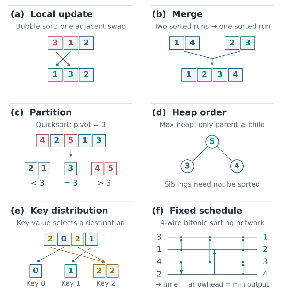
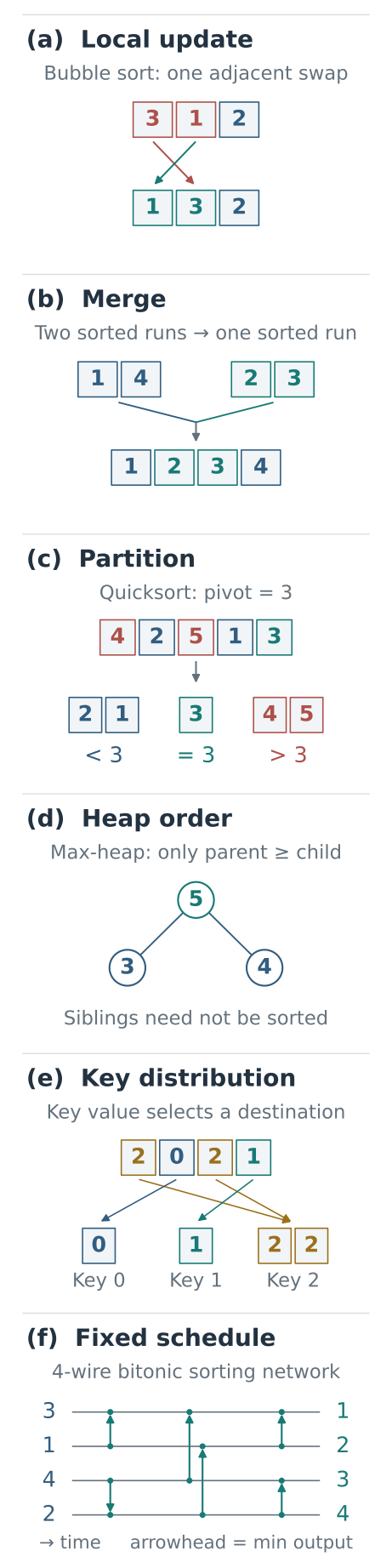
Figure 1. (a) Bubble sort swaps an inverted adjacent pair; the array is not yet sorted. (b) Merge combines two sorted runs; colors identify the source run. (c) Partition groups keys below, equal to, and above 3; the left group remains unsorted. (d) A max-heap orders each parent against its children, not the siblings against one another. (e) Key values select destinations. (f) A bitonic network sorts [3, 1, 4, 2] with six fixed comparators: time runs left to right, and each arrowhead receives the smaller value. Each panel uses its own example.
The phrase “binary sort” needs care. Binary insertion sort uses binary search to locate an insertion point. Binary heapsort uses a binary heap. Bitonic sort uses a comparison network. These are different algorithms; the word “binary” does not establish a time bound.
4. Brute force and random search
4.1 Bogosort: random trials and expected cost
A deliberately inefficient strategy is to shuffle the array until it is sorted. The test is easy; finding the answer by blind guessing is not.
For [3, 1, 2], the six candidates are [1,2,3], [1,3,2], [2,1,3], [2,3,1], [3,1,2], and [3,2,1]. Only the first is sorted. A fresh random guess can revisit any failed candidate; it does not cross that candidate off a list.
With $n$ distinct records, there are $n!$ possible permutations and exactly one ascending permutation. Suppose every shuffle is uniform and independent. One shuffle succeeds with probability
\[p=\frac{1}{n!}. \tag{5}\]For an initially unsorted input, let $X$ count shuffles up to and including the successful one. Then $X$ has a geometric distribution:
\[\begin{aligned} \Pr(X>m)&=(1-p)^m,\\ \mathbb E[X]&=\frac{1}{p}=n!. \end{aligned} \tag{6}\]One Fisher–Yates shuffle takes $\Theta(n)$ work. A sortedness scan takes at most $O(n)$; even if an unsuccessful scan stops early, the shuffle already costs linear work. The expected total is therefore $\Theta(n\,n!)$ for initially unsorted distinct-key inputs. If the initial array is already sorted, the first scan finishes in $\Theta(n)$ without shuffling.
The worst case is unbounded, not “$n!$ shuffles.” For every finite $m$, $(1-p)^m>0$: there is still a positive chance of failing that many times. Ideal independent shuffling terminates with probability one, but no finite number of shuffles guarantees success. With duplicate values, several labeled permutations may satisfy the key ordering, so the success probability changes.
The following bounded demonstration stops instead of hanging:
1
2
3
4
5
6
7
8
9
10
11
12
13
14
15
16
17
18
# Requires is_sorted from Section 1.
import random

def bogo_sort_bounded(a, max_shuffles=2000, seed=0):
    """Return (sorted copy or None, shuffles used); never change a."""
    if max_shuffles < 0:
        raise ValueError("max_shuffles must be nonnegative")
    a = list(a)  # Keep the caller's input intact.
    rng = random.Random(seed)
    for attempts in range(max_shuffles + 1):
        if is_sorted(a):
            return a, attempts
        if attempts < max_shuffles:
            rng.shuffle(a)
    return None, max_shuffles

result, attempts = bogo_sort_bounded([3, 1, 2])
assert result is None or result == [1, 2, 3]
The seed makes the experiment reproducible. A finite pseudorandom trace illustrates the probability model; it is not a proof that shuffles in the implementation are ideal independent random variables.
Shuffle until sorted: how long is n!?
Loading interactive model…
Model & data
Distinct keys 1..n, n=3..7; reverse input starts unsorted. Each attempt is a complete Fisher–Yates shuffle using the seeded 32-bit LCG (1664525x+1013904223 mod 2^32), for reproducible demonstrations. At most 2,000 attempts are generated; reaching the limit is not success. The theoretical success probability 1/n! and expected n! attempts assume independent uniformly random permutations; a finite pseudorandom seeded run is not that assumption or a worst-case guarantee. A shuffle takes Θ(n) writes; checking sortedness takes O(n), so the usual expected random-sort time is O(n·n!) under that model. No finite worst-case attempt bound exists for unbounded random shuffling.
Try increasing $n$ by one. The expected number of guesses multiplies by $n+1$, not by a fixed constant. The demonstration is capped at 2,000 attempts; reaching that cap means “not found within this budget,” not “no sorted order exists.”
4.2 Permutation sort: exhaustive enumeration
Exhaustive brute force avoids repeated guesses:
1
2
3
4
5
6
7
8
9
10
# Requires is_sorted from Section 1.
from itertools import permutations

def permutation_sort(a):
    # Only use tiny inputs: every candidate is a complete ordering.
    for candidate in permutations(a):
        if is_sorted(candidate):
            return list(candidate)

assert permutation_sort([3, 1, 2]) == [1, 2, 3]
For distinct keys, the correct permutation is somewhere in a list of $n!$ candidates. In the worst case it is last. Generating each length-$n$ candidate requires $\Theta(n)$ work in this implementation, giving worst-case $\Theta(n\,n!)$. Enumeration guarantees reaching the answer; it still discards almost every useful relationship learned from earlier candidates.
“Brute force” is a description of a strategy, not a formal algorithm name. Selection sort is also sometimes called a brute-force method, but its quadratic work is vastly smaller than enumerating permutations.
5. Selection sort: repeated minimum selection
Selection sort finds the smallest remaining record and places it at the front of the unsorted suffix.
On [4, 1, 3, 2], the first scan starts by treating index 0 as the best candidate. Comparing 1 with 4 changes smallest to index 1. Comparing 3 and then 2 with that candidate leaves it unchanged. Nothing moves during the scan; only the remembered index changes. The final swap places 1 at index 0.
The vertical bar separates finalized positions from the remaining search area:
1
2
3
4
5
       fixed | remaining
start        | 4 1 3 2
left=0     1 | 4 3 2
left=1   1 2 | 3 4
left=2 1 2 3 | 4
The remaining area can change dramatically, but the finalized prefix never needs revisiting.
1
2
3
4
5
6
7
8
9
10
11
12
13
14
15
16
def selection_sort(a, key=lambda x: x):
    """Sort a in place and return the same list; not stable."""
    for left in range(len(a) - 1):
        smallest = left
        for j in range(left + 1, len(a)):
            if key(a[j]) < key(a[smallest]):
                smallest = j
        # Everything before left is already final.
        if smallest != left:
            a[left], a[smallest] = a[smallest], a[left]
    return a

values = [4, 1, 3, 2]
result = selection_sort(values)
assert values == [1, 2, 3, 4]
assert result is values  # The caller sees the same modified list.
Selection, bubble, and insertion sort below modify the supplied list itself. Their return a returns that same list, not a separate sorted copy. range(len(a) - 1) visits left = 0 through n - 2; the final slot needs no search.
An invariant is a statement that holds at each iteration boundary. Here it is precise: before iteration left, the prefix contains the left smallest keys in sorted order. Initially the prefix is empty, so the statement holds without doing anything. The scan finds a minimum of everything else, so putting it next extends that prefix. When one element remains, it must belong in the last position.
The scans compare $n-1,n-2,\ldots,1$ pairs:
\[\begin{aligned} C(n)&=\sum_{j=1}^{n-1}j\\ &=\frac{n(n-1)}{2}\\ &=\Theta(n^2). \end{aligned} \tag{7}\]This count is unchanged by an already sorted input. Best, average, and worst comparison counts are all quadratic. There are at most $n-1$ swaps, so selection sort can make fewer record writes than insertion sort on a reversed array. “Same Big O” does not mean “same kind of work.”
The swap implementation is not stable. On [2a, 2b, 1], swapping the final 1 with 2a produces [1, 2b, 2a]. Choosing the first minimum with < does not prevent the distant swap from reversing equal records.
6. Bubble sort: adjacent comparisons and swaps
A left-to-right pass compares neighbors and swaps them when necessary. After one full pass, a largest remaining value is at the right end: it keeps moving right whenever it meets a smaller neighbor.
Use the same input, [4, 1, 3, 2]. Unlike selection sort, bubble sort changes the array immediately after a successful comparison:
1
2
3
4
5
6
7
8
9
pass 1:
4 1 3 2
1 4 3 2   swap 4,1
1 3 4 2   swap 4,3
1 3 2 | 4 swap 4,2
pass 2:
1 2 | 3 4
pass 3:
1 2 3 4   no swap; stop
After comparing positions j and j + 1, a maximum of the records encountered so far is at j + 1. The next comparison carries that maximum one step farther. This explains why the last position is final even though most earlier positions might still be wrong. The next pass excludes that position by decreasing end.
1
2
3
4
5
6
7
8
9
10
11
12
13
14
def bubble_sort(a, key=lambda x: x):
    """Stably sort a in place and return the same list."""
    for end in range(len(a) - 1, 0, -1):
        changed = False
        for j in range(end):
            if key(a[j]) > key(a[j + 1]):
                a[j], a[j + 1] = a[j + 1], a[j]
                changed = True
        # A pass with no swaps proves all remaining neighbors are ordered.
        if not changed:
            break
    return a

assert bubble_sort([4, 1, 3, 2]) == [1, 2, 3, 4]
The rightmost finalized suffix grows by one after each pass. The early-exit flag matters: on sorted input, one pass makes $n-1$ comparisons and no swaps, so best-case time is $\Theta(n)$. Reversed distinct values require all passes and $\Theta(n^2)$ work. Uniformly random distinct permutations also have quadratic expected work.
A no-swap pass is a proof, not a guess that the input looks almost sorted. Every neighboring pair in the remaining prefix was tested and found ordered. That prefix is therefore sorted; the finalized suffix already contains the largest records in order, so the entire array is sorted.
Only strict out-of-order pairs are swapped. Equal-key records never cross each other, so this implementation is stable.
The extra passes explain a practical weakness. If one very small record starts at the far right, a left-to-right pass moves it left by only one position. A nearly sorted-looking array can still require many passes. Insertion sort handles that particular situation much more directly.
7. Insertion sort: insertion into a sorted prefix
Insertion sort keeps a sorted prefix. It removes the next record, shifts larger records right, and fills the resulting gap.
For [4, 1, 3, 2], the three insertions are:
1
2
3
4
5
sorted  | unprocessed
4       | 1 3 2
1 4     | 3 2   (shift 4)
1 3 4   | 2     (shift 4)
1 2 3 4 |       (shift 4,3)
“Remove” is logical here: item = a[i] saves the record in a temporary variable; Python does not shorten the list. During the first insertion, shifting 4 right makes the raw array [4, 4, 3, 2], while item still holds 1. Treat index 0 as the current hole: its old contents no longer count as a live record. Writing item into that hole gives [1, 4, 3, 2]. The temporary duplicate is not a lost 1 or an extra record in the final answer; the current records are represented by the array excluding the hole, plus the held item.
1
2
3
4
5
6
7
8
9
10
11
12
13
def insertion_sort(a, key=lambda x: x):
    """Stably sort a in place and return the same list."""
    for i in range(1, len(a)):
        item = a[i]
        item_key = key(item)
        j = i - 1
        while j >= 0 and key(a[j]) > item_key:
            a[j + 1] = a[j]  # Shift right; the hole moves left.
            j -= 1
        a[j + 1] = item
    return a

assert insertion_sort([4, 1, 3, 2]) == [1, 2, 3, 4]
Before iteration $i$, positions $0$ through $i-1$ are sorted. The shifted records are exactly the trailing records in that prefix whose keys exceed the new key. Inserting after all the others produces a sorted prefix of length $i+1$. Equal records are not shifted, which preserves stability.
7.1 Inversions and input disorder
An inversion is an index pair in the wrong order:
\[\begin{gathered} I(A)=\#\{(i,j):\\ i<j,\ k(A_i)>k(A_j)\}. \end{gathered} \tag{8}\]For [3, 1, 2], the inversions are (3,1) and (3,2), so $I=2$. The sorted array has $I=0$. A reversed array of distinct keys has every pair inverted:
Swapping an inverted adjacent pair removes exactly one inversion. Their relation to every other record is unchanged: the two positions were adjacent. Thus an adjacent-swap algorithm needs at least $I$ such swaps to sort. Bubble sort makes exactly $I$ swaps, though it may spend additional comparisons looking for them.
The shared example has four inversions: (4,1), (4,3), (4,2), and (3,2). Its insertion trace makes $1+1+2=4$ shifts. Selection sort still makes six key comparisons; insertion sort’s shift work instead tracks the actual disorder.
Insertion sort makes exactly $I$ shifts of larger records. Each shift moves one earlier, larger record past the inserted record and resolves their inversion. It also performs $O(n)$ loop and final-placement work. Therefore its running time is
\[T(A)=\Theta(n+I(A)). \tag{10}\]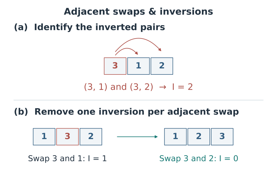
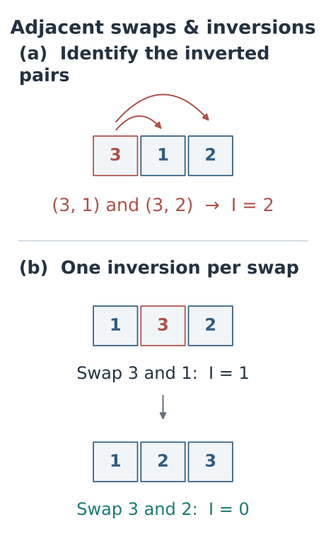
Figure 2. Swapping an inverted adjacent pair removes exactly one inversion. Insertion sort resolves the same pairwise disorder by shifting larger records past the record being inserted.
For a uniformly random permutation of distinct keys, each pair is inverted with probability $1/2$. Linearity of expectation gives
\[\mathbb E[I] =\frac12\binom n2 =\frac{n(n-1)}4. \tag{11}\]No independence between different pairs is needed for this expectation. This yields quadratic average-case time, while inputs with $I=O(n)$ take linear time. That is the mathematical reason insertion sort is useful for small or lightly disordered pieces inside more sophisticated algorithms.
Inversion game: remove the disorder
Loading interactive model…
Model & data
An inversion is an index pair i<j with a[i]>a[j]; equal keys do not count. Swapping adjacent inverted keys decreases I by exactly one; swapping an ordered pair increases I by one, and equal keys leave I unchanged. The manual board is separate from an insertion/binary-insertion trace regenerated from its current keys. Both stable variants shift exactly I records, but their writes also include one final placement for each inserted record. Binary search changes comparisons, not how many larger prefix records must move. Presets contain 4–5 keys. Animation counters and manual swap counts are separate.
Swap neighbors manually and compare the inversion count with the independent insertion trace. The trace counts final placements as well as shifts: for a nonempty length-$n$ input, its total record writes are $I+(n-1)$. Subtract the $n-1$ final placements to recover the shift count $I$. The number of inversions predicts shifts more accurately than the number of elements that “look misplaced.”
8. Binary insertion sort: search versus relocation
Binary search can locate an insertion point in the sorted prefix. It halves the interval of possible positions after each comparison, so finding a position among $i+1$ gaps takes $O(\log(i+1))$ comparisons.
To remain stable, the new record must go after existing equal-key records. The required search is an upper bound: the first position whose key is strictly greater than the new key, or the end if none exists. This is a binary-search position, not the asymptotic upper bound used in Big O.
For the sorted prefix [1, 2a, 2b, 4], inserting a new 2c must return index 3, not index 1 or 2. The labels distinguish equal-key records:
1
2
3
4
lo hi mid test      update
 0  4   2 2b <= 2c  lo=3
 3  4   3 4 > 2c    hi=3
 3  3     stop: insert at 3
The comparisons use only numeric keys. In [lo, hi), hi is an excluded record index, but inserting at hi remains a possible answer. Indices before lo have keys at most the new key; indices from hi to the prefix’s end have greater keys. Each update removes mid from the unresolved records: lo = mid + 1 or hi = mid. The interval strictly shrinks, so it reaches lo == hi. Then only 4 shifts right, producing [1, 2a, 2b, 2c, 4]. Binary search located the gap; shifting made room for it.
1
2
3
4
5
6
7
8
9
10
11
12
13
14
15
16
17
18
19
20
21
22
def binary_insertion_sort(a, key=lambda x: x):
    """Stably sort a in place using upper-bound insertion positions."""
    for i in range(1, len(a)):
        item = a[i]
        item_key = key(item)
        lo, hi = 0, i  # Search the half-open prefix [0, i).
        while lo < hi:
            mid = (lo + hi) // 2
            if key(a[mid]) <= item_key:
                lo = mid + 1  # Equal records stay before the new record.
            else:
                hi = mid
        # Finding lo did not create an empty slot: records must move.
        for j in range(i, lo, -1):
            a[j] = a[j - 1]
        a[lo] = item
    return a

records = [(2, "a"), (1, "a"), (2, "b")]
assert binary_insertion_sort(records, key=lambda x: x[0]) == [
    (1, "a"), (2, "a"), (2, "b")
]
Summing the binary-search costs gives $O(n\log n)$ key comparisons. But inserting at position zero still shifts the entire prefix. On reversed input, the total shifts remain
\[\begin{gathered} 1+2+\cdots+(n-1)\\ =\frac{n(n-1)}2\\ =\Theta(n^2). \end{gathered} \tag{12}\]For the code above, total time is $\Theta(n\log n+I)$. Even sorted input performs the binary searches, giving $\Theta(n\log n)$ time, unlike ordinary insertion sort’s linear best case. An additional “already follows the prefix” check could restore that best case, but it is not present here.
This is an important distinction: a faster search for a destination does not make relocation free. Binary insertion can be worthwhile when comparisons are expensive and moving references is cheap. It is not a general $O(n\log n)$ array sort.
9. Merge sort: divide, sort, and stable merge
Two sorted lists can be merged without repeatedly searching either one. Their smallest remaining records are at their fronts. Compare those two, output the smaller, and advance only the side that supplied it.
For [1, 4, 8] and [2, 3, 9], the successive choices are 1, 2, 3, 4, 8, then the remaining 9. Each record is copied once into the output. At most $p+q-1$ key comparisons merge nonempty lists of lengths $p$ and $q$.
Why is looking only at the fronts enough? Suppose those fronts are 4 and 2. Every remaining record in the first list is at least 4; every remaining record in the second is at least 2. Therefore 2 is a smallest remaining record overall. No search through the tails could find a smaller one. Sorted inputs let one comparison settle the next output position permanently.
The recursive calls create those sorted inputs; splitting alone does not sort anything. For four records, the complete dependency is:
1
2
3
4
5
split:  [7, 2a, 5, 2b]
        [7, 2a]       [5, 2b]
        [7] [2a]      [5] [2b]
merge:  [2a, 7]       [2b, 5]
        [2a, 2b, 5, 7]
The letters distinguish records with equal key 2; they are not part of the comparison. Calls descend until len(a) <= 1, then return their results to their waiting callers. In the final merge, left = [2a, 7] and right = [2b, 5]. Starting at i = j = 0, the comparisons choose 2a (advance i), 2b (advance j), and 5 (advance j again). Now right is exhausted, so out.extend(left[i:]) appends 7. The other extend appends nothing. This is why the code needs two read positions but never moves either backward.
1
2
3
4
5
6
7
8
9
10
11
12
13
14
15
16
17
18
19
20
21
22
23
24
25
26
def merge_sort(a, key=lambda x: x):
    """Return a stable sorted copy; leave a unchanged."""
    if len(a) <= 1:
        return list(a)
    mid = len(a) // 2
    left = merge_sort(a[:mid], key)
    right = merge_sort(a[mid:], key)
    out = []
    i = j = 0
    while i < len(left) and j < len(right):
        if key(left[i]) <= key(right[j]):
            out.append(left[i])  # Left wins ties: preserve stability.
            i += 1
        else:
            out.append(right[j])
            j += 1
    # Only one tail can be nonempty; its records are already sorted.
    out.extend(left[i:])
    out.extend(right[j:])
    return out

records = [(7, "a"), (2, "a"), (5, "a"), (2, "b")]
ordered = merge_sort(records, key=lambda record: record[0])
assert ordered == [(2, "a"), (2, "b"), (5, "a"), (7, "a")]
assert records == [(7, "a"), (2, "a"), (5, "a"), (2, "b")]
assert ordered is not records  # A new list; the input is unchanged.
The merge invariant says out is sorted and contains the smallest already consumed records from the two inputs. Neither unconsumed list can contain a smaller record behind its front. Once one side is exhausted, the other side is already sorted and can be appended.
The recursive proof follows by induction on length. Lists of length zero or one are sorted. If both smaller recursive results are correct, merging them returns a sorted permutation of the original list. Choosing the left record on ties keeps equal records from the earlier half ahead of equal records from the later half; recursion preserves their internal order.
9.1 Recurrence and the n log n bound
For $n=2^m$, splitting in half reaches single records after $m=\log_2n$ levels. A level contains many subproblems, but their lengths add up to $n$.
For eight records, the merge sizes are four pairs, then two groups of four, then one group of eight. These are three rounds, each handling eight records in total. Doubling the input to sixteen adds one round; it does not double the number of rounds. That repeated halving is the source of the logarithm. In general, the work per level is:
\[\begin{aligned} 1\times\Theta(n)&=\Theta(n),\\ 2\times\Theta(n/2)&=\Theta(n),\\ 4\times\Theta(n/4)&=\Theta(n). \end{aligned} \tag{13}\]Each line is $\Theta(n)$. There are $\log_2n$ lines, hence $\Theta(n\log n)$ total work. Equivalently,
\[\begin{gathered} T(n)=2T(n/2)+\Theta(n),\\ T(n)=\Theta(n\log n). \end{gathered} \tag{14}\]For lengths that are not powers of two, the halves differ by at most one; the depth is bounded by $\lceil\log_2n\rceil$ and the same asymptotic result holds.
The equation for $T(n)$ is a recurrence: it expresses the cost of one call using the costs of its smaller calls. The 2 counts those calls, not two complete sorts of the original array. The added linear term pays for the splitting and merging done by the current call. Counting the recursion tree by levels is one way to solve that recurrence without a separate theorem.
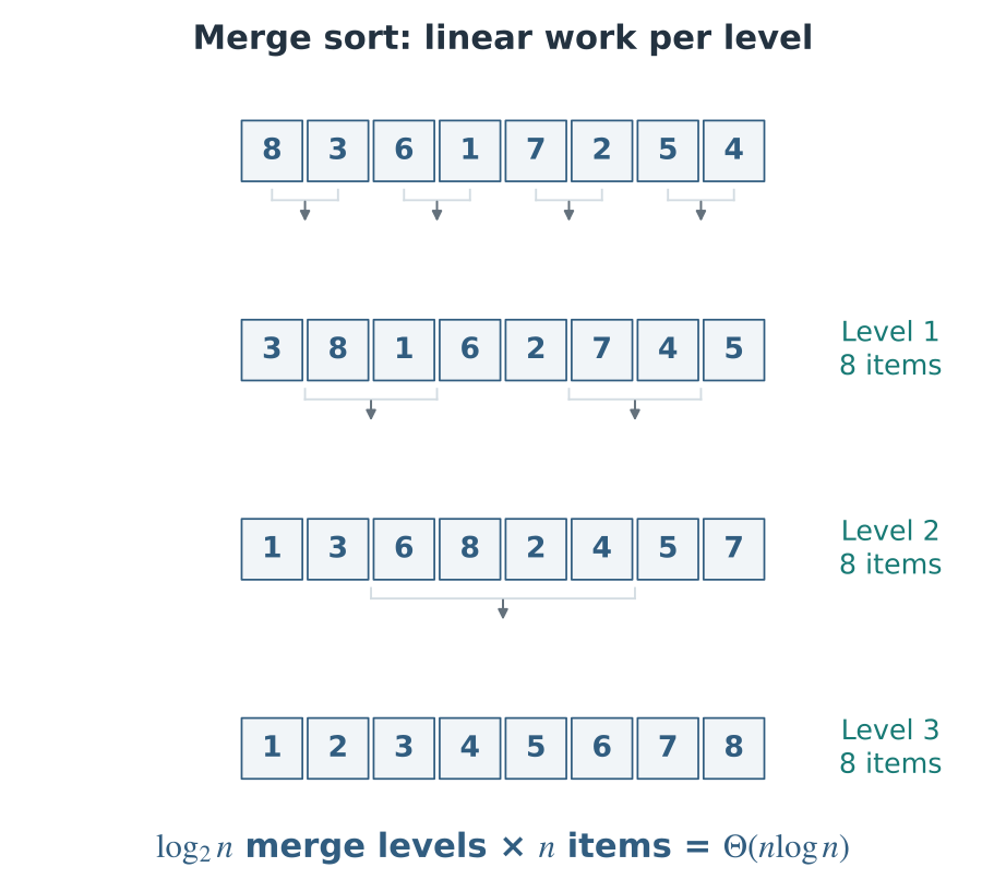
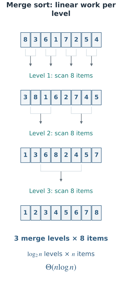
Figure 3. Each merge level handles eight records in total. The brackets identify the two input runs of each merge. For general input size $n$, balanced splitting produces $O(\log n)$ levels with $O(n)$ work per level.
The Python slices also copy records. They add $\Theta(n)$ work per level, not an extra multiplicative logarithm: the full recurrence already has a linear term at each level. This implementation takes $\Theta(n\log n)$ time even on sorted input, since it still splits, copies, and merges.
Peak auxiliary storage is $\Theta(n)$, including output lists and temporary slices; the recursion stack is $O(\log n)$. The total volume allocated over the entire run is $\Theta(n\log n)$, but those allocations are not all alive simultaneously. Peak memory and cumulative allocation are different quantities. These are the standard stable array-merge tradeoffs described in Princeton’s merge-sort reference.
A run is a contiguous sequence that is already sorted. The activity starts with two runs and asks you to choose their next output record.
Merge two runs: who wins a tie?
Loading interactive model…
Model & data
Original sequence is left run [2a,4,6a] followed by right run [2b,3,6b]. Each run is already sorted. Pick buttons append the selected run head even when it is the wrong next choice; sortedness and equal-key stability are then inspected independently. A stable merge takes the left head on equal keys because all original left-run records preceded the right run. Undo removes one pick. Complete stable merge applies the correct rule only to the remaining records; it does not undo an earlier incorrect pick. No key writes or comparisons are timed here.
Step through a merge with equal-key labels. Changing the tie decision may leave the numbers sorted while reversing equal records. The sortedness condition alone cannot detect that loss of stability.
10. Quicksort: random pivots and three-way partitioning
Merge sort divides by position, then combines the answers. Quicksort divides by key value: choose a pivot and separate records smaller than, equal to, and larger than it. The equal group needs no further sorting by that key.
10.1 Partition invariants and pointer updates
A three-way partition records which keys are already classified and which remain to be checked.
For a concrete partition, choose pivot key 3 in [4, 2, 3, 1, 5, 3]. This is a chosen-pivot example, not a trace promised for the function’s default random seed. The pointers start at lt = i = 0, gt = 5. Each row below records the state after the indicated action:
1
2
3
4
5
6
7
8
test   array          lt i gt
start  [4,2,3,1,5,3]   0 0 5
4 > 3  [3,2,3,1,5,4]   0 0 4
3 = 3  [3,2,3,1,5,4]   0 1 4
2 < 3  [2,3,3,1,5,4]   1 2 4
3 = 3  [2,3,3,1,5,4]   1 3 4
1 < 3  [2,1,3,3,5,4]   2 4 4
5 > 3  [2,1,3,3,5,4]   2 4 3
After the first swap, index 0 contains a newly arrived 3. Keeping i = 0 makes the next iteration classify it. Advancing i at that point would wrongly treat an unexamined record as known. By contrast, when 1 swaps with lt, the displaced 3 was already in the equal region, so advancing both pointers is safe. The last swap exchanges a slot with itself and still removes it from the unknown region.
At the end, [2, 1] is smaller than the pivot, [3, 3] equals it, and [5, 4] is larger. The side groups are not yet sorted. The calls sort(0, 1) and sort(4, 5) finish them. No later operation needs to move a record across the equal group.
The following interval notation states exactly what has become known at every step. A half-open interval such as [lo, lt) includes lo but excludes lt; it is empty when the endpoints coincide.
For the current record there are three actions. A smaller record is swapped into the left region; both lt and i advance. An equal record simply extends the middle region. A larger record is swapped into the right region; gt decreases, but i does not advance, because the record brought in from the unknown end has not been examined.
1
2
3
4
5
6
7
8
9
10
11
12
13
14
15
16
17
18
19
20
21
22
23
24
25
26
27
28
29
30
31
32
import random


def quick_sort_3way(a, key=lambda x: x, seed=0):
    """Sort a in place with random-pivot partitioning; return a."""
    rng = random.Random(seed)

    def sort(lo, hi):
        if lo >= hi:
            return
        # Choose a pivot from the inclusive interval [lo, hi].
        pivot = key(a[rng.randrange(lo, hi + 1)])
        lt, i, gt = lo, lo, hi
        while i <= gt:
            current = key(a[i])
            if current < pivot:
                a[lt], a[i] = a[i], a[lt]
                lt += 1
                i += 1
            elif current > pivot:
                a[i], a[gt] = a[gt], a[i]
                gt -= 1  # Recheck the incoming record at i.
            else:
                i += 1
        # The equal region is final. Only the two sides need sorting.
        sort(lo, lt - 1)
        sort(gt + 1, hi)

    sort(0, len(a) - 1)
    return a

assert quick_sort_3way([4, 2, 4, 1, 4, 3]) == [1, 2, 3, 4, 4, 4]
Every iteration shortens the unknown interval by one, so a partition of $m$ records takes $\Theta(m)$ time. The recursive calls handle only the smaller and larger groups. When those are sorted, concatenating the three regions is sorted without a merge. This is the same three-way invariant used in Princeton’s quicksort treatment.
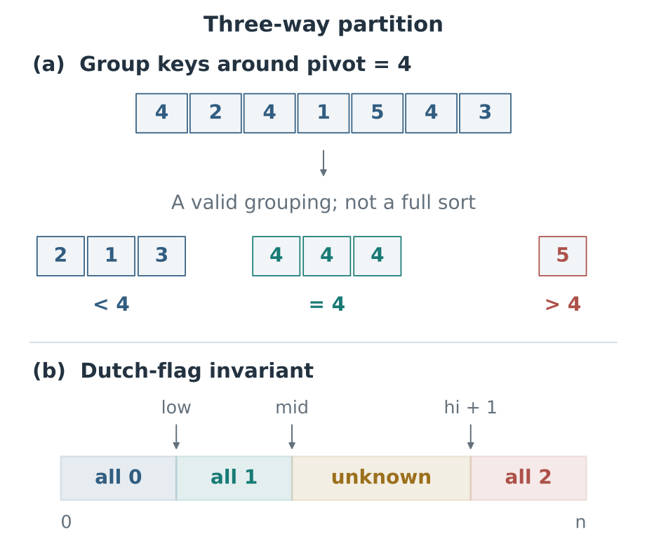
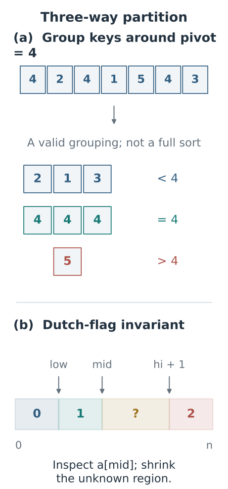
Figure 4. (a) A valid three-way grouping around pivot 4; each outer group still needs sorting. (b) The Dutch-flag specialization for keys 0/1/2 and pivot 1. Its unknown interval includes both mid and hi; hi+1 begins the finished 2 region.
10.2 Partition balance and expected time
If partitions repeatedly split distinct keys into comparable-sized pieces, the recursion has $\Theta(\log n)$ levels with $\Theta(n)$ work per level: $\Theta(n\log n)$ time.
If the pivot is repeatedly the smallest remaining key, one side is empty and the other has size $n-1$:
\[\begin{aligned} T(n)&=T(n-1)+\Theta(n),\\ T(n)&=\Theta\left(\sum_{m=1}^n m\right)\\ &=\Theta(n^2). \end{aligned} \tag{16}\]Uniform random pivot selection avoids tying this behavior to a particular input pattern, but it does not eliminate the worst possible random sequence. For every fixed distinct-key input, expected time is $\Theta(n\log n)$ under independent uniform pivot choices; the worst realization still takes $\Theta(n^2)$.
For eight distinct records, a repeatedly extreme pivot leaves sizes 8, 7, 6, ...: the same surviving records get scanned many times. A roughly central pivot instead leaves two groups of about half the size; both groups can shrink again at the next level. Random selection does not promise a central pivot on every call. Its benefit is that extreme pivots do not keep occurring predictably on a fixed input.
One way to see the expectation is to consider sorted ranks $i<j$. In ordinary randomized quicksort, they are compared only if the first pivot selected from ranks $i,\ldots,j$ is an endpoint. That event has probability $2/(j-i+1)$. Summing over pairs yields
\[\begin{aligned} \mathbb E[C_n] &=\sum_{1\le i<j\le n}\frac{2}{j-i+1}\\ &=2(n+1)H_n-4n\\ &=\Theta(n\log n), \end{aligned} \tag{17}\]where $H_n=\sum_{j=1}^n1/j=\Theta(\log n)$. This exact formula uses the standard distinct-key quicksort model with one comparison per pivot–record classification. It does not mean every possible pair is compared. The shown three-way Python code may make two key comparisons for a classification; its constant differs, but the expected order of growth does not.
For example, consider the records of sorted ranks 2 and 5. The relevant interval contains ranks 2, 3, 4, 5. If rank 3 or 4 becomes a pivot first, it separates the two records, which will never meet in a later recursive call. If rank 2 or 5 is first, it is compared with the other endpoint. Two of the four equally likely first pivots permit that comparison, giving probability $2/4$. The sum above adds these probabilities over pairs: an expected count can be computed without listing every possible recursion tree.
The logarithm in $H_n$ can be seen without calculus. Group the terms into blocks with indices 2–3, 4–7, 8–15, and so on. Each complete block contains a power-of-two number of terms and sums to between $1/2$ and $1$. There are $\Theta(\log n)$ such blocks; a final incomplete block adds at most one. Thus the whole harmonic sum has logarithmic growth.
With all keys equal, three-way partitioning handles the entire input in one linear pass and makes no nonempty recursive calls. Its best case over inputs allowing duplicates is therefore $\Theta(n)$, not $\Theta(n\log n)$. With distinct keys, balanced partitions give the latter best-case order.
The code mutates the input but needs a recursion stack: expected $O(\log n)$ depth for distinct keys, $O(n)$ in the worst case. Large pathological inputs can exceed Python’s recursion limit before completing. A production implementation can recurse on the smaller side and iterate over the larger one to bound stack depth. Distant swaps make this version unstable.
The next activity fixes the pivot at 1 and the keys at 0, 1, and 2, so the four regions can be inspected without recursive calls. Follow what arrives at the scan position after a 2 is swapped to the right. The final coding test uses this same invariant.
Dutch flag: shrink the unknown region
Loading interactive model…
Model & data
Array contains 2–24 keys, each 0,1,2. Invariants: [0,low) are 0; [low,mid) are 1; [mid,high] unknown; (high,n) are 2. A 0 swaps with low and advances low and mid. A 1 advances mid. A 2 swaps with high and decreases high without advancing mid, because the incoming value is unclassified. The unknown length high-mid+1 decreases by one each iteration, yielding exactly n iterations and at most 2n record-array writes with self-swaps omitted. This in-place partition is not stable. Visual snapshots are auxiliary teaching data, not algorithm workspace.
The general sorting playground in section 1 deliberately uses the first record as pivot, so input order can expose unbalanced splits. The Python function above uses random pivots for the expected bound. Do not transfer the expectation to a deterministic pivot rule without also specifying an input distribution. Duplicate-heavy data in that playground shows why separating the equal region matters.
11. Heapsort: heap construction and maximum extraction
A heap is not a fully sorted array. In a max-heap, every parent is at least as large as either child. This guarantees that the root is a maximum, while leaving many other pairs unordered.
In a zero-based array, index $i$ has children $2i+1$ and $2i+2$. The layout is a complete binary tree: all levels are full except possibly the last, which is filled from the left. Its height is $\Theta(\log n)$.
For [3, 1, 6, 5, 2, 4, 7], the root is index 0 with value 3; its children are indices 1, 2 with values 1, 6. Index 1 owns children 3, 4 with values 5, 2; index 2 owns children 5, 6 with values 4, 7. The array itself stores the tree—no node objects or links are needed.
Leaves at indices 3 through 6 already satisfy heap order because they have no children. Bottom-up repair starts at n // 2 - 1 = 2:
1
2
3
4
start:  [3,1,6,5,2,4,7]
root 2: [3,1,7,5,2,4,6]
root 1: [3,5,7,1,2,4,6]
root 0: [7,5,6,1,2,4,3]
The last repair first swaps 3 with the larger child 7, then swaps that 3 with 6 below it. Choosing the larger child matters: swapping with 5 would leave the other child 7 above the new parent value 5. Each chosen child is already the maximum of its own subtree, which is precisely the information needed to repair the next parent safely.
Extraction swaps the root 7 with the last active slot. The temporary array is [3, 5, 6, 1, 2, 4 | 7], where the bar separates the active heap from the finished suffix. Repair moves 3 below 6, then below 4, producing the first row below. Repeating extraction finishes the sort:
1
2
3
4
5
6
[6, 5, 4, 1, 2, 3 | 7]
[5, 3, 4, 1, 2 | 6, 7]
[4, 3, 2, 1 | 5, 6, 7]
[3, 1, 2 | 4, 5, 6, 7]
[2, 1 | 3, 4, 5, 6, 7]
[1 | 2, 3, 4, 5, 6, 7]
In sift_down(root, end), end is exclusive: the sorted suffix must never participate in a repair. Heap order identifies the next maximum without fully sorting the active region. For example, 5 and 4 can sit in separate branches; no comparison between them is needed until their relationship affects a root repair.
1
2
3
4
5
6
7
8
9
10
11
12
13
14
15
16
17
18
19
20
21
22
23
24
def heap_sort(a, key=lambda x: x):
    """Sort a in place using a max-heap and return a; not stable."""
    def sift_down(root, end):
        # [0, end) is the active heap. Children are already heaps.
        while 2 * root + 1 < end:
            child = 2 * root + 1
            if child + 1 < end and key(a[child]) < key(a[child + 1]):
                child += 1
            if key(a[root]) >= key(a[child]):
                break
            a[root], a[child] = a[child], a[root]
            root = child

    n = len(a)
    # Leaves need no repair. Build valid subheaps from bottom to top.
    for root in range(n // 2 - 1, -1, -1):
        sift_down(root, n)
    for end in range(n - 1, 0, -1):
        # Put the maximum into its final slot, outside the smaller heap.
        a[0], a[end] = a[end], a[0]
        sift_down(0, end)
    return a

assert heap_sort([3, 1, 6, 5, 2, 4, 7]) == [1, 2, 3, 4, 5, 6, 7]
During a sift, the root may violate heap order, but its child subtrees already satisfy it. Swapping with the larger child fixes the parent position; only the child’s new position can still be wrong. The process moves downward, eventually restoring the subtree. Bottom-up construction can therefore build on subheaps already repaired.
11.1 The linear cost of bottom-up heap construction
“$n$ nodes times $\log n$” is a valid upper bound but too loose. Most nodes cannot travel $\log n$ levels. Roughly half are leaves and travel zero; a quarter are at height one, an eighth at height two, and so on. The number of nodes of height $h$ is at most $n/2^{h+1}+1$. Summing their possible downward steps gives
\[\begin{gathered} T_{\mathrm{build}}(n)\\ =O\left(n\sum_{h\ge0}\frac{h+1}{2^{h+1}}\right)\\ =O(n). \end{gathered} \tag{18}\]The finite-tree rounding terms add only $O(\log^2n)$, which is also $O(n)$. The construction loop itself has $\Theta(n)$ iterations, giving $\Theta(n)$ build time. Repeated insertion into an initially empty heap is a different construction and has $O(n\log n)$ worst-case time.
After construction, there are $n-1$ root removals. Each repair takes at most $O(\log n)$, so heapsort has $O(n\log n)$ worst-case time; the worst-case bound is tight. It uses $O(1)$ auxiliary record storage and no recursion.
For this early-stopping sift implementation, all equal keys give linear total time: each repair stops immediately. With distinct keys, standard binary heapsort has $\Theta(n\log n)$ best-case as well as worst-case time. The duplicate distinction and bottom-up construction bound are documented in Princeton’s heap reference. Root-to-end swaps make the implementation unstable.
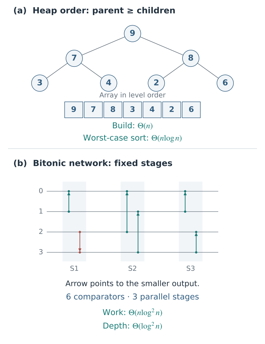
Figure 5. (a) A max-heap and its level-order array representation; each parent is at least as large as its children. (b) A four-wire bitonic network with six comparators in three stages. Comparator arrows point toward the smaller output; comparators in the same stage use disjoint wires.
12. The comparison-sorting lower bound
Suppose all $n$ keys are distinct and the algorithm learns their order only through comparisons. A comparison has two possible outcomes, so its choices can be drawn as a binary decision tree. A leaf specifies the final ordering selected by the algorithm.
With three input records named a, b, and c, the possible output orders are abc, acb, bac, bca, cab, and cba. The letters identify records, not known numerical ranks. One valid comparison strategy is:
1
2
3
4
5
6
7
8
9
10
11
a < b?
  yes: b < c?
         yes -> abc
         no: a < c?
               yes -> acb
               no  -> cab
  no:  a < c?
         yes -> bac
         no: b < c?
               yes -> bca
               no  -> cba
For a = 9, b = 2, c = 5, the answers are no, no, yes. They establish b < c < a, so the leaf outputs the records as bca, or [2, 5, 9]. Other inputs can finish after two questions, but some need three. Two yes/no questions can distinguish at most four outcomes, fewer than the six required; a clever rearrangement of the questions cannot avoid a third question somewhere.
There are $n!$ possible relative input orders. A correct algorithm must distinguish them: if two different orders reached the same leaf, the same output permutation would be used for both, and at least one would be wrong. A binary tree of height $h$ has at most $2^h$ leaves, hence
\[\begin{gathered} 2^h\ge n!,\\ h\ge\lceil\log_2(n!)\rceil. \end{gathered} \tag{19}\]The growth rate does not require memorizing Stirling’s formula. Since every factor is at most $n$,
\[\log_2(n!)\le n\log_2n. \tag{20}\]For even $n$, the last $n/2$ factors are each at least $n/2$:
\[\begin{aligned} n!&\ge(n/2)^{n/2},\\ \log_2(n!)&\ge\frac n2\log_2\frac n2. \end{aligned} \tag{21}\]The odd case differs only by rounding. Together these prove $\log_2(n!)=\Theta(n\log n)$, giving an $\Omega(n\log n)$ worst-case comparison lower bound. Merge sort and heapsort achieve that order, so the bound is tight. The comparison model and its limits are covered in MIT’s sorting lecture.
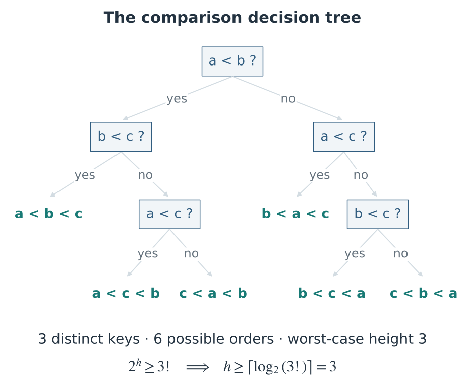
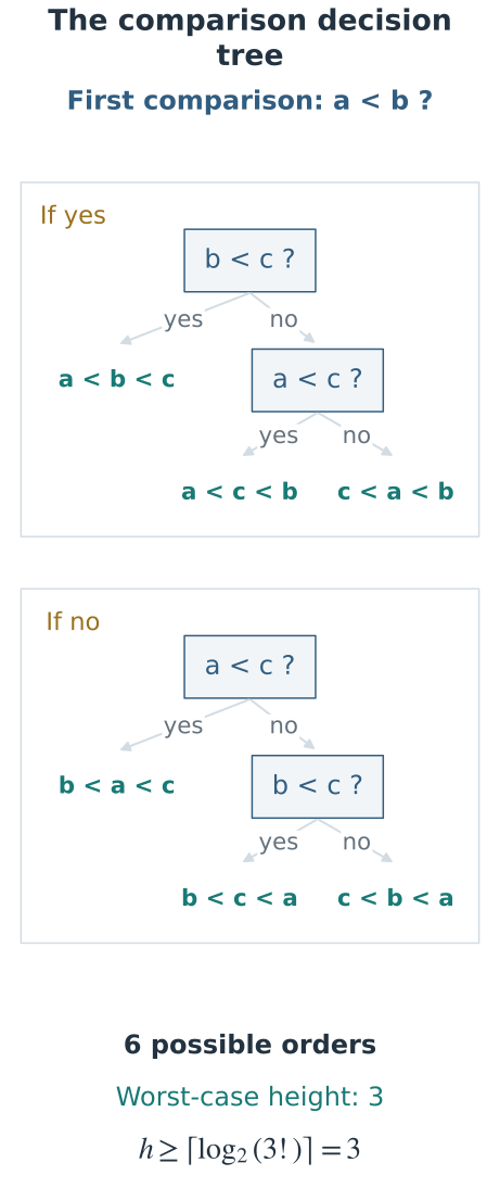
Figure 6. A comparison supplies at most one bit of binary decision information. Distinguishing $n!$ possible orders needs enough decisions, even with a clever choice of comparisons.
This does not say that every individual input requires $n\log n$ work. An algorithm may verify an already ordered input in linear time. It does not cover algorithms that inspect integer digits or use keys as array addresses. Under a uniform distribution of distinct relative orders, a corresponding average-depth argument also gives an $\Omega(n\log n)$ expected comparison bound. Randomization does not remove that general comparison-model barrier.
13. Counting sort: histograms, prefix sums, and stable scatter
If keys are integers in ${0,\ldots,K-1}$, the key can directly index an array. A histogram counts each key. Prefix sums then identify where records with that key belong.
For keys [2, 0, 2, 1, 0], the counts are [2, 1, 2]. The starting offsets are [0, 2, 3]: two zeros occupy positions 0–1, one one occupies position 2, and two twos occupy positions 3–4.
The counts answer how many records each key has. The offsets answer where their reserved space begins. These are different questions. To find the first slot for key 2, add the counts for keys 0 and 1, because all those records must precede every 2. Do not add the count for 2 itself: that would give the end of its reserved interval, not the beginning.
The tagged input in Figure 7 makes the placement step visible. Here 2a means a record with key 2 and identity a; the identity is carried along, not compared.
1
2
3
4
5
6
7
8
9
input: [2a,1a,2b,0a,1b]
count: [1,2,2]
start: [0,1,3]

2a -> 3: [ ·, ·, ·,2a, ·]
1a -> 1: [ ·,1a, ·,2a, ·]
2b -> 4: [ ·,1a, ·,2a,2b]
0a -> 0: [0a,1a, ·,2a,2b]
1b -> 2: [0a,1a,1b,2a,2b]
Each placement advances only that key’s next-free-slot cursor. After placing 2a, the cursor for key 2 changes from 3 to 4; 2b therefore goes immediately after it. The array next_slot begins with the offsets and then tracks the next available output position for each key. Its final contents are no longer the original starts.
1
2
3
4
5
6
7
8
9
10
11
12
13
14
15
16
17
18
19
20
21
22
23
24
25
26
def counting_sort(a, K, key=lambda x: x):
    """Return a stable sorted copy for integer keys in [0, K)."""
    if K < 0:
        raise ValueError("K must be nonnegative")
    count = [0] * K
    for item in a:
        value = key(item)
        if not isinstance(value, int) or not 0 <= value < K:
            raise ValueError("keys must be integers in [0, K)")
        count[value] += 1

    # Exclusive prefix sums: each key begins after all smaller keys.
    next_slot = [0] * K
    for value in range(1, K):
        next_slot[value] = next_slot[value - 1] + count[value - 1]
    out = [None] * len(a)
    for item in a:
        value = key(item)
        out[next_slot[value]] = item
        next_slot[value] += 1  # Advance this key's next free slot.
    return out

records = [(2, "a"), (1, "a"), (2, "b"), (0, "a"), (1, "b")]
assert counting_sort(records, 3, key=lambda record: record[0]) == [
    (0, "a"), (1, "a"), (1, "b"), (2, "a"), (2, "b")
]
For key $v$, its initial offset is
\[s_v=\sum_{u=0}^{v-1}\operatorname{count}[u]. \tag{22}\]Exactly $s_v$ records have smaller keys, so the records with key $v$ belong in the contiguous interval starting there. Scanning the input left to right and consuming positions in increasing order preserves the order of equal records. This proves stability as well as sortedness and the permutation condition.
This is an exclusive prefix sum: the sum stops before the current key. For the tagged example, exclusive starts are [0, 1, 3], whereas inclusive cumulative counts are [1, 3, 5]. Either convention can support a correct counting sort, but the scatter must match it. A common alternative uses inclusive counts as one-past-the-end positions, scans the input right to left, decrements the selected count, and then writes. Mixing that end-position convention with this left-to-right, increasing-cursor code would produce incorrect addresses or lose stability.
Two scans process $n$ records, and initializing and prefix-summing the arrays processes $K$ entries:
\[\begin{gathered} T(n,K)=\Theta(n+K),\\ S(n,K)=\Theta(n+K). \end{gathered} \tag{23}\]Calling this simply “linear time” is meaningful only when $K=O(n)$ or $K$ is otherwise controlled. Five IDs ranging from zero to one million still require a histogram with 1,000,001 slots in this direct implementation. A huge sparse key range is a poor fit even when $n$ is small.
Negative integer keys can be shifted: for a known minimum $m$, use key(item) - m and set $K=\max k-\min k+1$. This changes addresses, not relative ordering. A histogram alone can reconstruct plain integers, but keeping full records and stability requires a scatter such as the one above. The prefix-count/scatter pattern also underlies Princeton’s key-indexed counting and radix algorithms.
14. LSD radix sort: stable sorting by digit
Counting sort needs one slot per possible whole key. Radix sort instead processes a small part of the key at a time. In base $b$, digit $j$ of a nonnegative integer $x$ is
\[\operatorname{digit}_j(x) =\left\lfloor\frac{x}{b^j}\right\rfloor\bmod b. \tag{24}\]LSD means least significant digit first. Sort by the units digit, then tens, then hundreds, with each pass stable. Shorter numbers have leading zero digits.
For x = 237, place = 10, and base = 10, integer division gives 237 // 10 == 23: the units digit has been discarded. Taking 23 % 10 gives 3, the digit now at the right edge. With place = 1, the same expression gives 7; with place = 100, it gives 2. Multiplying place by base moves the operation one digit to the left without converting the number to a string.
1
2
3
4
5
6
7
8
9
10
11
12
13
14
15
16
17
18
19
20
21
22
# Requires the stable counting_sort from Section 13.
def radix_sort_nonnegative(a, base=10):
    """Return a sorted copy of nonnegative integers, one digit per pass."""
    if base < 2:
        raise ValueError("base must be at least 2")
    if any(not isinstance(x, int) or x < 0 for x in a):
        raise ValueError("expected nonnegative integers")
    out = list(a)
    if not out:
        return out
    maximum = max(out)
    place = 1
    while place <= maximum:
        out = counting_sort(
            out, base, key=lambda x: (x // place) % base
        )
        place *= base
    return out

assert radix_sort_nonnegative([170, 45, 75, 90, 802, 24, 2, 66]) == [
    2, 24, 45, 66, 75, 90, 170, 802
]
14.1 Stability and the induction over digits
Consider the four tagged records in Figure 7:
1
2
3
4
5
input:       [21a, 13a, 21b, 12a]
units keys:  [  1,   3,   1,   2]
after units: [21a, 21b, 12a, 13a]
tens keys:   [  2,   2,   1,   1]
after tens:  [12a, 13a, 21a, 21b]
After the units pass, the whole numbers are not sorted: 21 still precedes 12. That is expected. The pass promises only units-digit order. During the tens pass, both 12a and 13a enter the tens-1 group. Their earlier order, 12a before 13a, survives because the pass is stable. The tens digit now takes priority, while the units digit breaks ties. The equal whole keys 21a and 21b also retain their input order.
After the first pass, records are ordered by their lowest digit. Suppose that after $j$ passes they are ordered by their lowest $j$ digits. The next pass groups them by digit $j$. Different digit-$j$ values now have the correct higher priority. Within equal digit-$j$ groups, stability preserves the lower-$j$-digit order already established. Thus the records are ordered by their lowest $j+1$ digits. Induction proves the final numeric order.
For example, [12, 11] becomes [11, 12] after the units pass. Both have tens digit 1. An unstable tens pass could reverse them to [12, 11] and destroy the previous work. Stability is part of the proof, not an optional cosmetic feature.
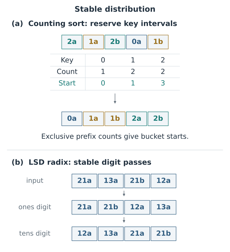
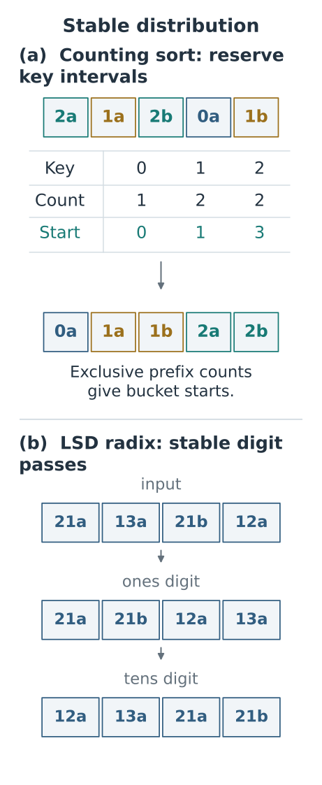
Figure 7. (a) Counts and exclusive prefix sums reserve an output interval for each whole key. (b) Stable ones- and tens-digit passes preserve the order established by lower digits. The labels follow the same records throughout.
With $d$ passes and radix $b$, the time is $\Theta(n+d(n+b))$, including the initial scan and copy. Peak auxiliary storage is $\Theta(n+b)$ when at least one pass is performed. For positive maximum $M$, $d=\lfloor\log_bM\rfloor+1$; the all-zero case performs zero digit passes and uses $\Theta(n)$ time and extra space. The common simplified time bound is
\[\begin{gathered} T(n,b,d)=O(d(n+b)),\\ d\ge1. \end{gathered} \tag{25}\]With fixed-width machine integers and a fixed digit width, $d$ and $b$ can be treated as constants, giving linear time in $n$. If integers may grow arbitrarily long, digit count and the cost of integer operations must be included. Increasing the radix reduces the number of passes but makes the histogram larger; memory and cache behavior help determine a useful radix.
For signed integers in a known range, subtracting a common minimum makes all keys nonnegative without changing their order. Fixed-width implementations can instead transform the sign-bit ordering appropriately. Treating an ordinary two’s-complement bit pattern as an unsigned magnitude without such a policy would put negative values in the wrong place.
Stable buckets: counting and LSD radix
Loading interactive model…
Model & data
2–16 keys in 0–99. Counting uses max(key)+1 buckets and appends records in input order. LSD radix uses base 2 or 10 and scans places 1,b,b²,… through the highest digit, preserving queue order in each bucket. Records are gathered back in increasing bucket order. Every bucket append and output slot assignment counts as a record-array write; count/index arithmetic is not counted. Empty buckets are omitted visually, but still contribute to K/base and the Θ(n+K) or Θ(d(n+b)) cost models. During output writing the main array may temporarily repeat identities because it is only partly overwritten; the complete buckets retain all records. These pedagogical queue buckets have Θ(n+K) space; this is not an in-place radix implementation.
Compare one whole-key counting pass with stable LSD passes in base 2 and base 10. Follow labeled equal digits through the scatter. A lower comparison count does not imply no work: histogram updates, prefix sums, and record writes still have a cost.
15. Bucket sort: interval partitioning and input distributions
Bucket sort distributes keys into ordered intervals, sorts each bucket, and concatenates the results. Unlike counting sort, a bucket can contain many distinct keys. An inner sorting algorithm is still needed.
For example, use four buckets for [0.78, 0.17, 0.39, 0.26, 0.72]. Their intervals are [0, 0.25), [0.25, 0.50), [0.50, 0.75), and [0.75, 1). Multiplying a key by four and rounding down selects its bucket: 0.39 goes to bucket 1 because floor(4 * 0.39) = 1.
1
2
3
4
5
6
7
8
9
after distribution:
bucket 0: [0.17]
bucket 1: [0.39, 0.26]
bucket 2: [0.72]
bucket 3: [0.78]

sort within bucket 1: [0.26, 0.39]
concatenate:
[0.17,0.26,0.39,0.72,0.78]
Distribution alone did not order 0.39 and 0.26; insertion sort still had to swap their local order. It did avoid comparing them with 0.72 and 0.78, because the interval boundaries already establish those relationships.
For values in $[0,1)$, $k$ equal-width buckets use index $\lfloor kx\rfloor$:
1
2
3
4
5
6
7
8
9
10
11
12
13
14
15
16
17
18
19
20
21
22
# Requires insertion_sort from Section 7 for each local bucket.
def bucket_sort_unit(a, bucket_count=None):
    """Return a sorted copy of values in [0, 1)."""
    n = len(a)
    if bucket_count is None:
        bucket_count = max(1, n)
    if bucket_count < 1:
        raise ValueError("bucket_count must be positive")
    buckets = [[] for _ in range(bucket_count)]
    for x in a:
        if not 0 <= x < 1:
            raise ValueError("expected keys in [0, 1)")
        buckets[int(bucket_count * x)].append(x)
    out = []
    for bucket in buckets:
        insertion_sort(bucket)
        out.extend(bucket)
    return out

assert bucket_sort_unit([0.78, 0.17, 0.39, 0.26, 0.72], 4) == [
    0.17, 0.26, 0.39, 0.72, 0.78
]
Everything in an earlier bucket is less than everything in a later bucket. Thus locally sorting every bucket makes the concatenation globally sorted. Stable insertion and left-to-right appending preserve equal-value order in this version; a record-capable extension uses the same key consistently for bucketing and local sorting.
Let $n_j$ be the occupancy of bucket $j$. Insertion-sorting the buckets costs at most a constant times $\sum_j n_j^2$, in addition to $O(n+k)$ distribution and concatenation work. If bucket indices are independent and uniformly distributed, then
\[\begin{gathered} \mathbb E\left[\sum_{j=0}^{k-1}n_j^2\right]\\ =n+\frac{n(n-1)}{k}. \end{gathered} \tag{26}\]To derive this, expand the sum as one contribution for each record and one for each ordered pair of distinct records landing in the same bucket. Each pair shares a bucket with probability $1/k$. Consequently, expected time is
\[O\left(n+k+\frac{n^2}{k}\right). \tag{27}\]Choosing $k=\Theta(n)$ yields expected $\Theta(n)$ time under those assumptions. Independence and uniform occupancy are doing real work in the proof. If every value lands in one bucket in reversed order, insertion sort in that bucket takes $\Theta(n^2)$. Uniform marginal bucket probabilities without independence are not enough to justify the same pair calculation.
The squared bucket sizes explain why distribution matters. With eight records, eight singleton buckets contribute 8 * 1² = 8 to the bound; two buckets of size four contribute 2 * 4² = 32; one bucket of size eight contributes 8² = 64. These are terms in a work bound, not exact comparison counts. Uniform randomness does not promise singleton buckets, but Equation (26) shows that their total squared occupancy stays linear in expectation when the number of buckets grows proportionally to the number of records.
The three distribution methods use different information. Counting reserves one region for an exact whole-key value. Bucket sort reserves one region for an interval and finishes the ordering locally. Radix sort repeatedly distributes by one digit; stability carries earlier digit information into later passes. Their linear-time claims therefore need different assumptions, not just the absence of comparison operators in a loop.
16. Hybrid sorts: combining strategies
16.1 Python sorting: runs, Timsort, and Powersort
For ordinary Python code, use sorted(records, key=...) or records.sort(key=...). The former returns a new list; the latter modifies the list and returns None. The key function is evaluated once per input record, and Python guarantees stable sorting. These are documented API properties, not properties of the short educational functions above. Python Sorting HOWTO.
1
2
3
4
5
6
7
students = [
    {"name": "Mina", "score": 90},
    {"name": "Joon", "score": 75},
    {"name": "Ara", "score": 90},
]
ordered = sorted(students, key=lambda student: student["score"])
assert [student["name"] for student in ordered] == ["Joon", "Mina", "Ara"]
A run is an already ordered contiguous section. An adaptive merge sort can discover runs, extend short ones with insertion-based work, and merge them instead of pretending every record starts unordered. If the entire list is a single run, recognizing it takes linear time. This explains how a comparison sort can have a linear best case while retaining an $O(n\log n)$ worst case.
For a small run-based example, consider [1, 4, 7, 2, 3, 8, 6, 5]. There are two ascending runs, [1, 4, 7] and [2, 3, 8], followed by the descending run [6, 5]. Reversing the last one gives [5, 6]. Merge the first two runs to obtain [1, 2, 3, 4, 7, 8], then merge that result with [5, 6]. The initial order inside each run has been reused rather than reconstructed through singleton merges. This illustrates the family of methods, not the exact run-extension or merge decisions a particular Python version would make on this eight-record input.
Extending a short run means taking additional records immediately after it and inserting them into its sorted region until a chosen minimum run length is reached, or the input ends. It does not mean padding with made-up keys. There is still insertion work, but it is confined to small pieces; later merges then avoid handling a large number of tiny runs.
A descending-run reversal needs a stability policy. Reversing [3a, 3b, 2a] directly produces [2a, 3b, 3a], reversing the equal 3 records. A simple stable design reverses only strictly descending runs. CPython 3.14 can also handle equal-key sections within descending runs by reversing those sections before reversing the whole run, restoring their original order. The simple rule and that optimized policy solve the same stability problem in different ways. CPython’s run handling.
Python documentation calls its algorithm Timsort. CPython 3.14 is a stable adaptive, run-based merge sort with a Powersort merge strategy, rather than the original Timsort merge policy unchanged. The design also includes techniques such as galloping during merges. Worst-case auxiliary storage is $O(n)$ even though list.sort() changes the original list. CPython 3.14 sorting design.
For nonempty input, the number $r$ of initial runs gives another way to think about adaptivity. If $r$ equal-sized runs are merged in a balanced tree, at most $\lceil\log_2r\rceil$ merge levels suffice, with $O(n)$ work per level, plus the initial scan. That idealized merge plan takes $\Theta(n+n\log r)$ time. Unequal run lengths require a suitable merge policy; simply counting runs does not specify which merges are efficient.
16.2 Introsort: bounding quicksort’s worst case
Introsort starts with quicksort-style partitioning but tracks recursion depth. If the partition tree grows too deep, it switches the affected subproblem to heapsort. Small pieces can use insertion sort. The original approach is described on David Musser’s author page.
The depth budget is a count of partition steps along a branch, not a timer. With a hypothetical budget of four, an eight-record subproblem that repeatedly leaves sizes 7, 6, 5, then 4 has consumed its budget without shrinking well. The remaining four-record piece is heapsorted instead of allowing the same bad pattern to continue. Real thresholds normally scale with the original input size rather than using this fixed illustrative number.
The depth threshold is chosen proportional to $\log n$. Before the switch, there are only $O(\log n)$ partition levels, each with at most $O(n)$ total work. The fallback heapsorts operate on disjoint remaining pieces; their combined work is at most $O(n\log n)$. This preserves a worst-case guarantee without giving up quicksort’s useful partitioning behavior. The exact threshold and implementation details are library choices, not part of the word “sort.”
At a single depth, the active subarrays do not overlap, so their lengths sum to at most $n$. That is why the partition work per level is linear even when there are many recursive calls. If the fallback pieces have lengths $m_1,m_2,\ldots$, each $m_i\le n$, and their total length is at most $n$. Bounding each $m_i\log m_i$ by $m_i\log n$ gives the same global $O(n\log n)$ cap for all fallback sorts together. The guarantee is built from a bounded number of partition levels plus bounded fallback work, rather than an assumption that the pivots will improve eventually.
Hybrid algorithms are useful because workloads contain several kinds of structure at once: tiny partitions, duplicate keys, existing runs, and expensive comparisons. A single textbook method need not handle every scale best.
17. Sorting networks, gap sequences, and alternative models
Bitonic networks, Shell sort, stooge sort, and sleep sort
17.1 Bitonic sort: comparator depth and total work
A comparator takes two values and outputs their minimum to one wire and maximum to the other. A sorting network fixes all comparator locations in advance; the pattern does not depend on the input values. Disjoint comparators in one stage can run simultaneously.
A bitonic sequence first rises and then falls, up to a cyclic rotation. Bitonic merging compares records separated by half the block size, then recursively handles the halves. A full bitonic sorting network repeatedly creates and merges these structures. NIST’s bitonic-sort entry describes its parallel formulation.
The four-wire network in Figure 5 uses three stages. Wire indices are fixed positions 0 through 3; records move between them. An ascending comparator puts the smaller value at the smaller index, while a descending comparator puts the larger value there. The trace abbreviates these directions as up and down.
1
2
3
4
5
6
7
input: [3,1,4,2]
stage 1: (0,1) up; (2,3) down
         [1,3,4,2]  bitonic
stage 2: (0,2) up; (1,3) up
         [1,2 | 4,3]
stage 3: (0,1) up; (2,3) up
         [1,2,3,4]
Stage 1 deliberately gives the two pairs opposite directions. Stage 2 compares positions half a block apart and sends each smaller value to the lower half. For a bitonic input, this split has the useful property that every value in the lower half is no larger than every value in the upper half; each half is itself bitonic and can be processed recursively. Merely comparing opposite positions would not establish that separation for an arbitrary input. Creating the bitonic structure first is essential. In the four-record example, only one final pairwise stage is needed to sort the two halves internally.
1
2
3
4
5
6
7
8
9
10
11
12
13
14
15
16
17
18
def bitonic_four(values):
    """Return a sorted copy using the fixed six-comparator network."""
    if len(values) != 4:
        raise ValueError("this network has exactly four wires")
    a = list(values)
    stages = [
        [(0, 1, True), (2, 3, False)],  # Build opposite-order pairs.
        [(0, 2, True), (1, 3, True)],   # Split the bitonic block.
        [(0, 1, True), (2, 3, True)],   # Finish each half.
    ]
    for stage in stages:
        for i, j, ascending in stage:
            if (ascending and a[i] > a[j]) or (not ascending and a[i] < a[j]):
                a[i], a[j] = a[j], a[i]
    return a

assert bitonic_four([3, 1, 4, 2]) == [1, 2, 3, 4]
assert bitonic_four([2, 1, 2, 1]) == [1, 1, 2, 2]
This Python loop executes all six comparators sequentially. Hardware with enough independent comparison units can execute the two disjoint comparators in each stage together, reducing six comparator operations to three dependent stages. Both counts describe the same network, but they measure different resources.
For $n=2^q$, the standard bitonic network’s number of dependent stages is
\[\begin{aligned} D(n)&=1+2+\cdots+q\\ &=\frac{q(q+1)}2\\ &=\Theta(\log^2n). \end{aligned} \tag{28}\]Each stage has $n/2$ comparators, so total work is
\[\begin{aligned} W(n)&=\frac n2D(n)\\ &=\Theta(n\log^2n). \end{aligned} \tag{29}\]With sufficient processors and the assumed communication model, the parallel depth can be logarithm-squared. A sequential machine must still execute all those comparators. Calling bitonic sort simply “$O(\log^2n)$” without saying parallel depth confuses two different resources. Its regular structure can suit hardware and some GPU workloads even though its sequential comparison count exceeds merge sort’s. Non-power-of-two lengths need an appropriate network or safe padding.
17.2 Shell sort: gapped insertion and gap sequences
Shell sort insertion-sorts records separated by a gap $g$, then reduces the gap until the final gap is one. Large gaps can move a record far with one relocation, avoiding insertion sort’s restriction to resolving nearby disorder.
With gap 4, an eight-record array has four interleaved subsequences at indices (0,4), (1,5), (2,6), and (3,7). Sort each subsequence as if it were a little array. It remains in its original strided positions; the records are not collected into contiguous groups.
1
2
3
4
input: [8,7,6,5,4,3,2,1]
gap 4: [4,3,2,1,8,7,6,5]
gap 2: [2,1,4,3,6,5,8,7]
gap 1: [1,2,3,4,5,6,7,8]
After gap 2, the even positions contain [2, 4, 6, 8] and the odd positions contain [1, 3, 5, 7]. The array is 2-sorted, not fully sorted. A gap-one pass finishes it, and in this example each misplaced pair is now only one position apart. Earlier passes did extra work so that the final insertion pass has less long-distance movement left.
1
2
3
4
5
6
7
8
9
10
11
12
13
14
15
16
17
18
19
20
21
22
def shell_sort_halving(a, key=lambda x: x):
    """Sort a in place with halving gaps and return a; not stable."""
    gap = len(a) // 2
    while gap > 0:
        for i in range(gap, len(a)):
            item = a[i]
            item_key = key(item)
            j = i
            # Insertion sort, but neighbors are gap positions apart.
            while j >= gap and key(a[j - gap]) > item_key:
                a[j] = a[j - gap]
                j -= gap
            a[j] = item
        gap //= 2
    return a

assert shell_sort_halving([8, 7, 6, 5, 4, 3, 2, 1]) == list(range(1, 9))
assert shell_sort_halving([]) == []
tagged = [(2, "a"), (2, "b"), (1, "a"), (3, "a")]
assert shell_sort_halving(tagged, key=lambda record: record[0]) == [
    (1, "a"), (2, "b"), (2, "a"), (3, "a")
]
That last assertion demonstrates instability rather than endorsing it. With gap 2, the 1a record pushes 2a from index 0 to index 2, past 2b at index 1. The final gap-one insertion pass does not reverse equal keys again. Strict comparisons preserve order within each individual gap subsequence, but cannot preserve it between different subsequences.
The final gap-one pass guarantees correctness, since it is an ordinary insertion sort. The speed depends strongly on the gap sequence. There is no single tight complexity bound that applies to every algorithm called Shell sort. A sequence consisting only of gap one is just insertion sort; useful sequences do more work before that final pass so that less remains. Shell sort is generally unstable, because equal records can cross through different gap subsequences. Princeton’s elementary-sort chapter includes gap-based sorting alongside insertion and selection.
The simple halving sequence in the code is an easy implementation, not a promise of an $n\log n$ worst case. It has $\Theta(\log n)$ passes, but each pass contains insertion loops whose cost depends on the remaining disorder. Even already sorted input takes $\Theta(n\log n)$ time here because every gap pass still scans the array; ordinary insertion sort would finish that input in $\Theta(n)$. Counting the number of gap values without analyzing the work inside each pass misses exactly the issue that made a nested loop expensive earlier.
For a conservative upper bound, a gap-$g$ pass sorts $g$ subsequences of roughly $n/g$ records each. Quadratic insertion work inside them sums to $O(n+n^2/g)$. Across halving gaps, the reciprocals sum to a constant: reading the gaps backward, they grow by at least a factor of two. This gives a total upper bound of $O(n\log n+n^2)=O(n^2)$; it does not establish an $O(n\log n)$ bound. Better gap sequences require their own analysis; long-distance movement is an opportunity, not a complexity proof by itself.
17.3 Stooge sort: overlapping recursion
Stooge sort compares the endpoints, then recursively sorts the first two thirds, the last two thirds, and the first two thirds again. Its correctness relies on overlapping subproblems, but that overlap is expensive:
For three records, those pieces are simply positions (0,1), then (1,2), then (0,1) again. Starting from [3, 1, 2], the endpoint comparison first gives [2, 1, 3]; the first two-record sort gives [1, 2, 3], and the other two sorts leave it unchanged. On larger inputs, the second recursive call can move smaller records into the overlap, so the first part must be sorted again. The third call is not an accidental duplicate: it repairs order that the second call may disturb. That repeated work is also why the method is slow.
Integer subproblem sizes use ceilings; these do not change the exponent. At recursion depth $\ell$, there are $3^\ell$ calls on pieces of size about $n(2/3)^\ell$. Reaching constant size takes $\log_{3/2}n$ levels. The number of leaves is therefore $3^{\log_{3/2}n}=n^{\log_{3/2}3}$. The geometric sum of call counts has the same order.
This is worse than quadratic. Recursion does not imply divide-and-conquer efficiency; the number, size, and overlap of subproblems determine the work.
17.4 Sleep sort: timers, scheduling, and key magnitudes
The joke is to launch one task per number, make it sleep proportionally to that value, and print when it wakes. It delegates ordering to timers, scheduling, and output synchronization. Close values can wake in the wrong order; negative keys, huge ranges, timer resolution, and thread creation need additional policies.
For [3, 1, 2] and a delay of one second per unit, ideal simultaneous tasks would print 1 after one second, 2 after two, and 3 after three. Changing just the largest value to one billion changes the waiting time to about 32 years, although the input still contains only three records. This exposes the hidden parameter: elapsed time depends on key magnitude, not merely on the number of records. Reducing the delay scale makes scheduling and timer errors harder to distinguish from genuine key differences.
This is not a general linear-time replacement for comparison sorting. It changes the machine model and charges elapsed time according to key magnitudes rather than just $n$. Timing services and parallel resources are not free sorting oracles.
18. Performance comparison and algorithm selection
The following table describes the specific implementations above under unit-cost keys. “Random distinct” means a uniformly random permutation of distinct keys. Bounds for integer methods include their extra parameters. Auxiliary space includes returned output and recursion stacks but excludes the given input.
| Method | Best time | Random distinct / expectation | Worst time | Extra space | Stable? |
|---|---|---|---|---|---|
| Selection | $\Theta(n^2)$ | $\Theta(n^2)$ | $\Theta(n^2)$ | $O(1)$ | No |
| Early-exit bubble | $\Theta(n)$ | $\Theta(n^2)$ | $\Theta(n^2)$ | $O(1)$ | Yes |
| Insertion | $\Theta(n)$ | $\Theta(n^2)$ | $\Theta(n^2)$ | $O(1)$ | Yes |
| Binary insertion | $\Theta(n\log n)$ | $\Theta(n^2)$ | $\Theta(n^2)$ | $O(1)$ | Yes |
| Slicing merge | $\Theta(n\log n)$ | $\Theta(n\log n)$ | $\Theta(n\log n)$ | $\Theta(n)$ | Yes |
| Random-pivot three-way quick | $\Theta(n)$ with equal keys | $\Theta(n\log n)$ expected for each fixed distinct input | $\Theta(n^2)$ | Expected $O(\log n)$ stack; worst $O(n)$ | No |
| Binary heap, early-stop sift | $\Theta(n)$ with equal keys | $\Theta(n\log n)$ | $\Theta(n\log n)$ | $O(1)$ | No |
| Stable counting | $\Theta(n+K)$ | Same parameterized bound | $\Theta(n+K)$ | $\Theta(n+K)$ | Yes |
| LSD radix | $\Theta(n+d(n+b))$ | Same for fixed $d,b$ | Same parameterized bound | $O(n+b)$ | Yes |
| Insertion-bucket | $\Theta(n+k)$ for already ordered buckets | Expected $\Theta(n)$ for independent uniform buckets and $k=\Theta(n)$ | $\Theta(n^2+k)$ | $\Theta(n+k)$ | Yes |
The quicksort expectation is over pivot randomness, not the input column’s distribution. For quicksort and heapsort restricted to distinct keys, the best-case time is $\Theta(n\log n)$. For bucket sort, $k$ denotes the number of buckets, not the key function; $K$ in counting sort denotes the number of possible integer keys. Empty and one-record inputs are trivial boundary cases rather than a different asymptotic growth law.
A useful selection rule is to ask what information is available. For general Python records, the stable built-in is the default. If the integer range is small, counting may remove comparison work. Fixed-width integer keys can suit radix passes. Data too large for memory favors designs that merge sequential streams, since memory transfers can dominate comparisons. If only a few extremes are needed, maintaining a heap can avoid fully sorting the input.
Stability, memory, worst-case requirements, and the cost of a comparison can matter more than a small difference in average comparison count. Benchmarks should use the same records, key policy, input distributions, and output requirements; timing one toy integer array cannot establish a universal winner.
19. Exercises: stability, complexity, and invariants
The five questions test different parts of a sorting argument: the output contract, a lower bound on work, the regions left after partitioning, a key-range assumption, and a loop invariant. Each question supplies its input diagram and assumptions. Check the relevant condition before choosing an answer; a numerically sorted array, for example, need not be stable or satisfy a one-pass classification contract.
Selecting an option shows why that particular choice succeeds or fails. A hint points to the condition to inspect without supplying the answer. Previous/Next preserves selections; Reset clears them. The diagrams below use the same inputs for working on paper.
Sorting concepts: five illustrated problems
Loading interactive model…
Model & data
Five fixed inputs test the sorting/stability contract [2a,1a,2b], the minimum adjacent-swap count for [4,3,2,1], 3-way quicksort on [4,4,4,4], direct-address counting with range 0..1,000,000 and n=5, and a Dutch-flag update at [1,2,0]. Each problem states its allowed operations and names the concept being tested. Hints do not reveal the option; a choice reveals both option-specific feedback and the full reasoning. Previous/Next preserves selections; Reset clears all answers and hints. Suffixes identify records, not secondary sort keys. Choices stay in the current browser activity and are not submitted.
Printable question diagrams
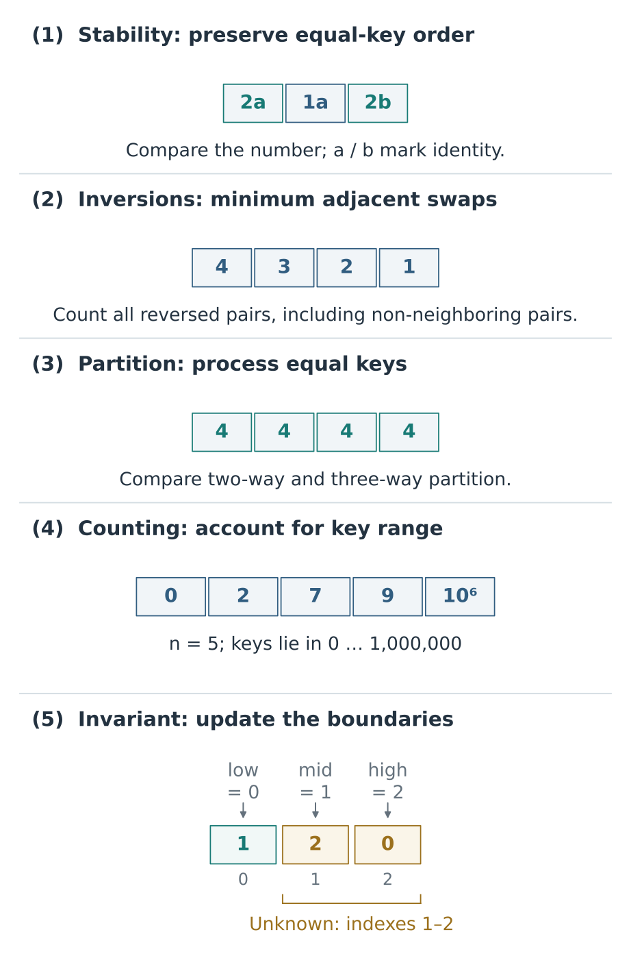
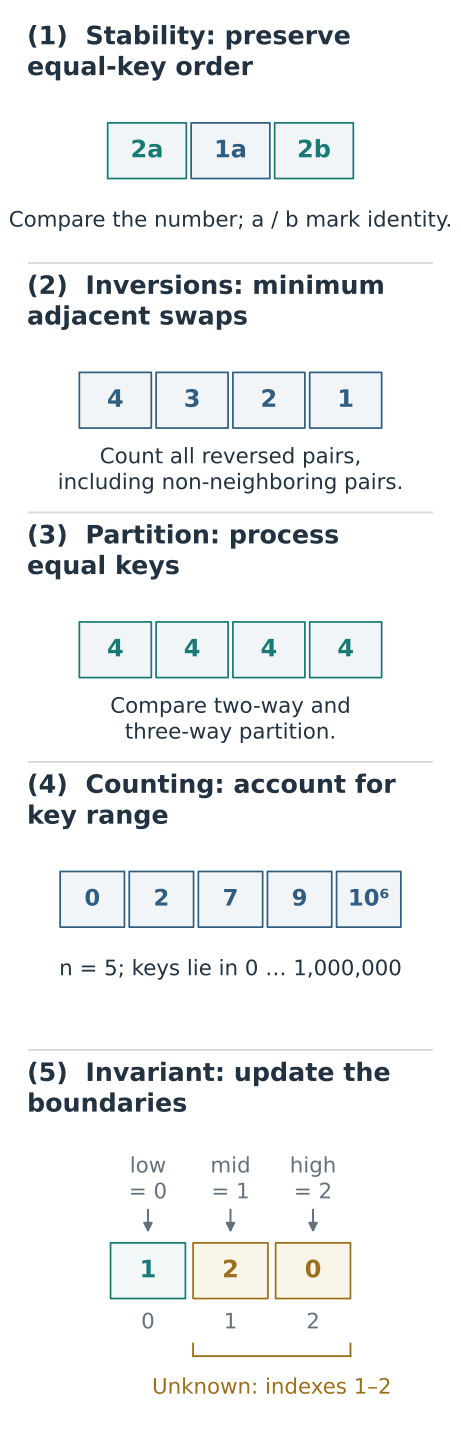
Figure 8. Record labels and region boundaries expose mistakes that an unlabeled final array would hide. The questions use the same inputs in the interactive workbench.
20. Coding test: implement the Dutch national flag
An array contains only 0, 1, and 2. Rearrange it in ascending order in place, using $O(1)$ extra storage and one classification pass. Do not call a sorting function. Counting and rewriting is a valid two-pass linear solution, but the one-pass constraint asks for the partition invariant itself.
For example, [2, 0, 2, 1, 1, 0] must become [0, 0, 1, 1, 2, 2]. Empty inputs, a single color, and repeated colors are all valid. Relative order within a color is not required. The function must modify and return the original list object; allocating a replacement list does not meet that API.
The Dutch national flag partition is the three-way partition with fixed pivot 1. Maintain zeros, ones, unknown records, and twos:
The code has three decisions to complete: whether the unknown interval includes its endpoints, whether the scan advances after placing a zero, and whether it advances after moving a two to the end.
Sort Colors: complete the partition invariant
Loading interactive model…
Model & data
Guided Sort Colors decisions, not arbitrary Python execution. Choose the loop condition and whether each 0-swap/2-swap advances mid; low always advances for 0 and high always decreases for 2. The compact Python outline omits the browser runner's counters and finite safety guard. Eight exact cases cover empty, singleton, sorted, reverse, recheck [1,2,0], all-2, mixed and a 24-record cycle. Expand each result for the tested concept, actual/expected arrays, terminal pointers, work counts and diagnosis. Each run stops after at most n iterations or on an invalid pointer invariant. Pass requires sorted output, an empty unknown interval, iterations<=n and writes<=2n; LIMIT is not success. Self-swaps count zero writes. The common API mutates and returns the original list. Visual trace snapshots are not algorithm workspace. The downloadable Python starter is fully runnable with the same three editable decisions and built-in counters; some initial cases intentionally fail.
The browser evaluates those bounded decisions against eight cases; it does not execute arbitrary Python. Each result expands to show the input, actual and expected output, final pointers, iteration count, and record writes. A FAIL may mean that the last record was never classified even though the numbers happen to be sorted. LIMIT means the iteration safety budget was reached; INVARIANT identifies invalid pointer relationships.
The Python starter is runnable with counters and safety checks already connected. Some of its three marked decisions are deliberately wrong; review TODOs 1–3, fix the incorrect choices, and rerun the tests. The same starter, fixtures and a separate reference solution are in the notebook. Three of the eight cases pass with the initial choices, so a few successful examples are not enough: all eight must pass, and the invariant must explain why the rules work for every legal input.
Reference solution and termination proof
1
2
3
4
5
6
7
8
9
10
11
12
13
14
15
16
17
18
19
20
21
def sort_colors(a):
    """Sort 0/1/2 in place in one classification pass; return a."""
    low = mid = 0
    high = len(a) - 1
    while mid <= high:
        if a[mid] == 0:
            a[low], a[mid] = a[mid], a[low]
            low += 1
            mid += 1
        elif a[mid] == 1:
            mid += 1
        elif a[mid] == 2:
            a[mid], a[high] = a[high], a[mid]
            high -= 1  # The incoming value at mid is still unknown.
        else:
            raise ValueError("colors must be 0, 1, or 2")
    return a

assert sort_colors([2, 0, 2, 1, 1, 0]) == [0, 0, 1, 1, 2, 2]
assert sort_colors([]) == []
assert sort_colors([2, 2, 0]) == [0, 2, 2]
When a zero is swapped with a[low], that incoming record is a known one if low < mid, or the same zero if the indices coincide. Advancing both pointers is therefore safe. When a two is swapped with a[high], the incoming record came from the unknown interval and might be zero, one, or two; advancing mid would skip its classification.
Define the number of unknown records as
\[U=\mathrm{high}-\mathrm{mid}+1. \tag{32}\]Initially $U=n$. Every valid branch reduces $U$ by exactly one, while preserving the four-region invariant. After exactly $n$ classification iterations, $U=0$. The remaining regions are zeros, ones, and twos in that order, and swaps have preserved all records. This proves $\Theta(n)$ time and $O(1)$ extra space.
The algorithm is linear because it classifies each record into a fixed set of three regions. It does not contradict the comparison lower bound for arbitrary distinct keys. That lower bound’s $n!$ possible orders are absent here.
The recurring question behind sorting speed is: what uncertainty does this operation remove? A neighboring swap fixes one inversion. A merge uses existing order to place a whole level’s records in linear work. A partition rules out cross-region comparisons. A heap keeps just enough order for repeated extraction. Counting and radix methods use key structure that comparisons alone cannot access. Their different bounds follow from those different sources of information.
References
- Sedgewick and Wayne, elementary sorting methods: selection, insertion, Shell sort, and implementation conventions.
- Princeton Merge API: a stable merge implementation with time and space bounds.
- Sedgewick and Wayne, quicksort: partitioning and equal-key handling.
- Sedgewick and Wayne, priority queues: binary heaps, bottom-up construction, and heapsort.
- MIT 6.006, lower bounds and linear-time sorting: the comparison model, counting, and radix sorting.
- Princeton string-sorting lecture: key-indexed counting and LSD radix sorting.
- Python Sorting HOWTO: stable sorting, key functions, and the public Python interface.
- CPython 3.14 sorting design: adaptive runs, merge policy, and memory behavior.
- David Musser, generic algorithms: the original introspective sorting approach.
- NIST Dictionary of Algorithms and Data Structures, bitonic sort: sorting-network and parallel terminology.