RSNA Knee, Part 6: A Technical Review of the Leading Solutions

Select a figure to enlarge it. On small screens, wide tables and equations scroll horizontally.

The strongest RSNA Knee systems did more than fit a better image classifier. They redesigned the chain between an MRI examination and a training target: what counted as a positive finding, which images a labeler could inspect, how uncertainty became a probability, where the classifier should collect evidence, and which parts of a radiology report reflected local practice rather than the image-defined task.

That chain matters because the competition did not provide ordinary supervised training data. Each MRI study needed twelve predictions, but only 58 of the 4,407 training studies came with expert image labels. Most studies instead had a multilingual radiology report. The test annotations were made by radiologists looking at images. An accurately extracted report was therefore a useful source of supervision without necessarily being an accurate representation of the test target.

The post-competition solutions make several differences measurable. The 21st-place author held the image learner fixed and replaced training labels; both a large weak-reference panel and the small expert panel improved. The 72nd-place author deliberately removed a site-related component at inference, improving Private while pooled report-reference OOF fell. The winning team supplied anatomy and lesion annotations to feature aggregation rather than relying only on study-level probabilities. Other teams found that more external images, more distillation rounds, or more blend variants did little. These are different experiments, and their results answer different questions.

My own work contained several of the same ingredients: multimodal labeling, wrong-image controls, native-field and local-view readers, teacher targets, complete OOF families, and whole-bank combination searches. The weakness was not that I lacked a list of standard techniques. I did not turn those ingredients into as strong a prediction basis. At the deadline, my strongest completed own-only composition scored Private 0.941; the public H system scored 0.942, and my selected mixture scored 0.943. I described the score trajectory and personal aftermath in the final retrospective. I needed to improve the information reaching the learner, evaluate the change against an appropriate reference, and let that result change the next research priority.

The source collection contains 38 solution accounts from 36 teams, alongside 51 archived notebook source bundles. Two accounts describe different parts of the same winning team. Numerical ablations below are the authors’ reports; static inspection of published code verifies selected operators and input paths, not an independent reproduction of those scores. Local label AUC, local student AUC, Public AUC, and Private AUC retain their separate meanings throughout.

Reading the score types

Macro ROC AUC gives each of the twelve findings the same weight, regardless of how common it is. For one finding, AUC measures how often a positive study is ranked above a negative study, with half credit at a tie. It is not a classification accuracy at threshold 0.5, and an improvement of 0.01 is not a claim that one percent more patients were diagnosed correctly.

An out-of-fold prediction is produced by an image model that excluded the evaluated study and the required group from its training partition. The reference used to score it may still be a constructed weak label. Public and Private are separate hidden evaluation subsets; the Private values in these reports were revealed after the deadline. The 58 expert-labelled training studies are a development resource, not the Private set.

An individual finding can also mean different things in these comparisons. A label table supplies a target value; a model learns from those values; an evaluator may threshold a reference table before computing AUC; the final competition evaluates against expert annotations. A higher number at one of those stages is not automatically an improvement at the others. The distinctions are especially important when comparing a ten-finding label evaluation with a twelve-finding model score, or a five-fold family with one full-data checkpoint.

1. Clinical targets and supervision

Clinical criteria and report-derived supervision

The twelve outputs did not describe twelve equally simple yes/no questions. ACL and MCL injuries, medial and lateral meniscus tears, three osteoarthritis compartments, effusion, synovitis, Baker’s cyst, contusion, and fracture required different anatomy, contrasts, and positive thresholds. A report could correctly describe an abnormality while failing to establish the particular target. Conversely, an expert reviewing the images for the competition could record a finding that had not been worth mentioning in the original clinical report.

The fifth-place team documented the discrepancy unusually well. The host rubric counted MCL injury at the acute high-grade partial or complete-tear level, yet the starting labels marked 199 reports describing low-grade MCL abnormalities as positive. Among five such examples in the expert set, none was positive; the corresponding fraction for other report-positive MCL cases was nine of thirteen. For effusion, ten of twenty-two reports describing small effusions were expert-positive, versus twenty-four of twenty-eight other report-positive effusions. These tiny subgroups do not establish universal clinical rates. They establish that treating every occurrence of a diagnostic term as the same supervision was an inadequate task definition.¹²

Finding or group	Distinction in the competition task	Failure of a literal report target
MCL injury	Acute high-grade partial or complete injury versus lower-grade changes	A correctly extracted low-grade abnormality can become a wrong positive target
Effusion and Baker’s cyst	The competition’s size threshold, rather than any visible fluid or cyst	“Trace” and “small” cannot automatically be merged with rubric-positive cases
Compartmental OA	The required extent of cartilage damage, attached to the correct compartment	A generic OA statement can conceal severity and medial/lateral/patellofemoral distinctions
Synovitis and effusion	Separate findings with overlapping but non-identical evidence	Inferring one from the other can manufacture label correlation

The second-place report gives the opposite side of the same problem. Across the 58 expert-labelled studies, the experts marked 240 positives where the reports explicitly stated 154. For patellofemoral OA the counts were twenty-one and two. Perfect extraction could not recover information that the text did not contain. Rephrasing a prompt to be more medically precise would help only when the necessary information was actually available to it.³

The targets needed to distinguish an explicit negative, an abnormality below the competition threshold, and an unmentioned finding. An unreadable or missing model response added a fourth state: annotation-pipeline failure. Collapsing them into one value made the training objective depend on how the table happened to encode missing information.

The fifth-place team found no answer for 27% of study–finding pairs in one starting public table, rising to 84% for synovitis. A value of 0.5 could represent uncertainty, failed extraction, or a missing-value convention. Under soft-target BCE, all such entries actively pull the prediction toward 0.5. A masked entry contributes no gradient, while an explicit negative pushes toward zero. Those states require different training instructions, even if a table initially stores them as the same default.

For example, with a presence mask $m_{i,c}$, a nonnegative confidence weight $w_{i,c}$, target $q_{i,c}$, and prediction $p_{i,c}$, a masked objective can be written as

\[\mathcal L= \frac{\sum_{i,c}m_{i,c}w_{i,c}\, \ell_{\mathrm{BCE}}(q_{i,c},p_{i,c})} {\sum_{i,c}m_{i,c}w_{i,c}}.\]

The denominator is assumed positive. Setting $m_{i,c}=0$ means no supervision for that entry. Leaving $m_{i,c}=1$ and choosing a low nonzero probability instead asserts a belief about disease in that group. That belief can be useful, but it needs a basis in the task and the population rather than a parsing convenience.

Four sources of information beyond the report

“External information” covers several different interventions. Additional knee MRIs enlarge or change the image population. Pretrained encoders, segmenters, and VLMs contribute knowledge learned elsewhere. Re-reading the competition’s own images adds supervision to existing examples. Teacher predictions transform information already captured by an image model. They have different costs, ancestry, and implications for evaluation.

Several strong systems used no additional MRI training studies. The seventh-place author used the competition data with ImageNet-pretrained backbones; the eighth-place account likewise reported no extra MRI data. The twenty-first-place author used OAI and KneeMRI for diagnostic comparisons, outside the final training pool. The twenty-second-place solution used ImageNet weights and a pretrained anatomical segmenter while reporting no external training data or other participants’ public prediction weights. Those uses of pretrained knowledge remain important even when an account reports “no external data.”⁴⁵⁶⁷

The second-place system did use external material: fastMRI with fastMRI+ information for parts of the encoder and orientation pipeline, and OAI MOAKS cartilage grades for a patellofemoral specialist. Those are meaningful advantages to investigate, but their role was more specific than appending a large dataset and expecting the competition metric to improve. A target-specific head can exploit an external clinical grading scheme even when that scheme does not match all twelve competition labels.

The more common supervision change was to let a stronger reader examine the competition’s MRI itself. A classifier that uses only images at inference can still benefit from reports, VLM reasoning, expert examples, and spatial annotations during training. This is privileged training information: expensive evidence acquisition happens once when targets are built, instead of being repeated for every hidden-test study.

My image-assisted labels had already tested this direction on a limited scale. A second report extraction might reduce translation or parsing errors, but inspecting the relevant images could recover findings absent from the text. A teacher could smooth uncertain targets and capture image patterns, yet also retain errors inherited from its report-derived training labels. These sources differ in the evidence they can add, not merely in the provider or model name.

Image coverage, reinspection, and report anchoring

Image-assisted supervision depended on the whole annotation system: the images available, the selection policy, the target definitions, the response format, and the instructions for using the report. Changing the API alone did not define the intervention.

The second-place team’s first pilot showed forty-four of 134 slices and suggested that images would not help. The later Astra pass saw every slice, approximately 277 images per study, together with the report and the text reader’s answers. The report was presented as a colleague’s interpretation with known gaps. Label AUC on the 58 expert cases rose from 0.899 for report reading to 0.942. Effusion improved from 0.806 to 0.975, and Baker’s cyst from 0.803 to 0.979. Because both reader and input policy changed, the comparison supports the complete annotation recipe rather than an isolated effect of adding slices.³

The winning team’s two annotation generations give a more controlled reason not to equate “multimodal” with a finished design. Sakaku’s earlier readers saw a fixed twenty-one-slice packet: seven sagittal, seven coronal, and seven axial images. ClinFusion supplied diagnostic explanations; Hulu used constrained yes/no token probabilities; Qwen produced continuous probabilities after reasoning. The final Astra reader instead began with overviews and could request neighboring slices, crop and window adjustments, and corresponding locations in another sequence. Its production budget was ten tool calls and ten detailed image sheets per study. DICOM geometry proposed corresponding locations, but the reader still had to verify the anatomy.⁸

A matched 224-pixel CoAt comparison already using multimodal Hulu-plus-Sol labels improved Public AUC from 0.922 to 0.935 after replacement with Astra labels. The gain cannot be explained as introducing images into a text-only pipeline. It concerns the quality of image-informed supervision after images were already present. The saved session’s seven calls and eight sheets are also not directly comparable with the approximately 277 individual images in the second-place input: a sheet, a slice, and a tool call are different counting units.

The twenty-first-place reader solved access differently. It browsed all series in pages of four previews, then retrieved native-resolution PNGs with crops or window adjustment when necessary. Its early instruction made an explicit report-positive statement force probability 1. Removing that instruction allowed image evidence and the competition definition to overrule the text. In the twenty-second-place protocol, each series became a montage—eighteen sagittal tiles or twelve coronal/axial tiles—with metadata supplied separately. That reader treated the report as an unverified reference. Adaptive tool use was therefore one way to address coverage, not a requirement shared by every successful pipeline.⁶⁷

Solution	Visual access and framing	What the comparison supports
1st, sakaku	Overviews plus bounded slice/crop/window and cross-sequence requests	A stronger complete multimodal label recipe after an earlier multimodal baseline
2nd	Approximately 277 images per study; report as a fallible colleague	Reader plus broader coverage improved expert-set agreement
7th	Structured, image-only, and verification reads	The same reader benefits from different evidence/framing channels, with target-specific failures
8th	Images and supporting locations first; report reviewed afterward	Image-first assessment can reduce anchoring before disagreement review
21st / 22nd	Full-series paging / metadata-supported montages	Broad coverage need not require the same interface or call budget

The seventh-place comparison was especially informative because it used one shared target protocol with three reads. Structured report-plus-key-slice reading scored 0.935 on gold-58; reading all images without the report scored 0.919; verification with the report treated as a possibly erroneous draft scored 0.947. The three-read blend reached 0.949, but the verification channel overcalled synovitis and effusion. Their prevalence rose from 0.24 to 0.31 and from 0.37 to 0.48. Excluding verification for those two findings reduced the label AUC slightly to 0.947, yet retained the more defensible target structure.⁴

The eighth-place team separated evidence acquisition into stages. Astra first saw images without reports or existing labels. Probabilities at least 0.5 required cited slices and boxes. Reports were then used to identify discrepancies, with another image review where necessary. The eventual image weight varied substantially: five-sixths for fracture, synovitis, and Baker’s cyst, but one-sixth for patellofemoral OA, lateral OA, and MCL. These weights were selected using the small expert set, so they are recipe choices rather than an independent ranking of which findings VLMs understand best. They nevertheless contradict a blanket rule that images should replace report targets everywhere.⁵

The thirty-second-place solution made a similarly selective correction. For 847 non-gold study–finding cells in site-associated disagreement groups, it replaced a normal 50/50 report/image target with the image reading alone. Other targets stayed unchanged. The author reported improved submission ordering while both displays remained at 0.960. This was a focused hypothesis about a particular subset, not evidence that increasing the image share globally was beneficial.⁹

The sixty-fifth-place account adds an important counterpoint to full-study reading. It divided the findings into anatomical groups and rendered twelve to thirty-two carefully selected slices per group. Effusion and synovitis used sagittal overview, sagittal zoom, and axial zoom sheets; the marrow group combined fluid-sensitive views with non-fat-suppressed images for fracture lines. The lateral group restricted sagittal input to the lateral third and used coronal joint crops. These choices changed the spatial information available to the annotator before any model response was generated.¹⁰

A single call covering ten findings with ninety images cost four to five times as much, yet lateral OA and patellofemoral OA each fell by about 0.08 in the development comparison. Smaller target-specific packets removed irrelevant material and retained detail that a dense contact sheet could obscure. The later fracture workflow used local zoom and boxes for 748 uncertain studies, concentrating the expensive read where it was needed.

Its reader comparison also separated standalone quality from complementarity. On the 54 expert cases left after each group’s four prompt references were excluded, Astra’s lateral OA AUC was 0.962 compared with 0.886 for text, while Opus 5.5 was only 0.574. Yet for synovitis, text scored 0.820, Astra 0.808, and Opus 0.822. The Opus–text combination reached 0.883. A generic ranking of the providers would have hidden the most useful pairing. The final reader choice reflected the finding, its crop, the available budget, and its contribution beside the existing text source.

The prompt included gold examples; when one of those examples was itself read, its reference was swapped. This prevented direct access to that case’s answer in the call, but the same cases had still informed prompts, exemplars, reader assignments, and mixtures. The 54-case scores therefore describe development performance, with the protocol and its failures available for inspection.

The report relationship also differed from the seventh-place verification approach. The sixty-fifth-place author found that image reads made with the report could look strong alone but contribute less after combining with the text source, whereas blind reads offered more complementary errors. The seventh-place result favored verification for most findings. These accounts need not contradict each other: the useful object is the complete reader–evidence–combination pipeline. A source that is excellent by itself can be redundant when its report information is already present in the target mixture.

The limits were equally informative. The seventy-fourth-place author accepted some image readers only for particular findings; removing crop and zoom from Opus 5.5 reduced its image-reading score from 0.726 to 0.693. The seventy-seventh-place account found no advantage for a multi-step tool-based reader over a simple report-plus-montage prompt. The 129th-place account reported direct image reading at about 0.73 on gold, against roughly 0.92 for its text labels. Visual access helped only when the reader, presentation, and target definition made that information usable.¹¹¹²¹³

Probability values as training instructions

A label source can preserve the correct order while producing poor probabilities. ROC AUC observes ordering; soft-target training also observes the numerical distance between the target and the current prediction. For a logit $z$, prediction $p=\sigma(z)$, and target $q$,

\[\ell_{\mathrm{BCE}}(q,p)=-q\log p-(1-q)\log(1-p), \qquad \frac{\partial\ell_{\mathrm{BCE}}(q,\sigma(z))}{\partial z}=p-q.\]

At prediction 0.8, targets 0.55 and 0.95 produce gradients of +0.25 and −0.15. They move the same student’s prediction in opposite directions. A strictly increasing transform preserves a finished label table’s AUC within a finding, but it does not preserve the objective optimized by a finite, regularized student.

The winning team therefore inspected log loss and confident errors alongside AUC. Tascj’s base reader and out-of-fold trained guide both scored approximately 0.936 label AUC, while log loss changed from 0.329 to 0.307 and confident errors from thirty-five to nineteen. A guide applied on the same expert examples used to fit it scored 0.943, which was explicitly separated from the fold-excluded comparison. The later reported temperature map was approximately $q^{\prime}=\sigma(0.77\operatorname{logit}q)$ for probabilities strictly between zero and one. A positive temperature preserves ordering; its purpose here was to alter the strength of the supervision.¹⁴

Sakaku’s output comparison was even more striking. On the same acquired evidence, an earlier six-bin readout scored 0.8832 development AUC versus 0.9363 for continuous outputs; a fresh complete continuous run scored 0.9392. This does not prove that all discrete schemes fail. The second-place reader successfully used categories plus a 0–100 score mapped by code into soft labels. The failure mode is loss of useful distinctions through a particular representation, not the mere presence of a category field.

The twenty-first-place labels supply a different diagnostic. Their AUC improved from 0.89576 to 0.93493 and Brier error from 0.13941 to 0.10396, while F1 at threshold 0.5 fell from 0.75013 to 0.72823. Better ranking and probability error did not imply a better fixed binary threshold. Converting such targets to hard labels because F1 was lower would discard the property the student was intended to learn.⁶

Confidence weights introduce another modeling decision. For fixed nonnegative weights, with any presence mask absorbed into $w$, the ideal unconstrained learner under weighted BCE has the following optimum at $x$.

\[p_w^*(x)=\frac{\mathbb E[wQ\mid X=x]}{\mathbb E[w\mid X=x]}, \qquad \mathbb E[w\mid X=x]>0.\]

Giving uncertain reports less weight can reduce unreliable gradients. It can also emphasize conspicuous findings and conventional phrasing, changing the effective conditional target. “Confidence” is not necessarily the probability that the annotation is correct, particularly when it is generated by the same reader that generated the label. Label content, target scale, missingness masks, and example weights should therefore be distinct entries in a comparison, rather than one undifferentiated label-cleaning operation.

Calibration from report groups to expert criteria

The fifth-place team began with two public report tables, including the table I had released. Its initial calibration, calA, adjusted soft targets to match expert-positive frequencies, fitting each validation fold’s adjustment from expert cases in the other folds. With training and inference held fixed, a CoAtNet’s Private AUC improved from 0.916 to 0.926. This is a direct matched example of useful information being recovered from an existing public label source. A later EfficientNetV2-M improvement from 0.946 to 0.954 combined a new label recipe with twenty-five rather than seventeen epochs; that difference cannot all be attributed to calibration.¹

One observation explained why a global correction was insufficient. Report-positive labels around 0.75 arising from hedged or low-grade findings were confirmed only 38% of the time. Synovitis inferred from effusion received the same value as explicitly described synovitis, around 0.84, while expert confirmation was 38% versus 65%. A score-only transform has no way to treat the same input value differently in the two groups. Group membership therefore supplies information that a global remapping lacks.

The thirty-eighth-place team made this approach explicit. It classified report statements into rubric-positive, below-threshold, uncertain, negative, and unmentioned groups, with quoted evidence and severity. Across the inspected gold study–finding pairs, the unmentioned group was positive in 9/144, explicit negatives in 9/197, mild or borderline findings in 32/96, and the rubric-positive group in 128/150. Those are pooled diagnostic counts across findings, not 144 independent studies or universal probabilities for each disease.¹⁵

Report group	Observed expert-positive pairs	Implication for target construction
Unmentioned	9 / 144, approximately 0.06	Silence was often negative in this sample, but neither exactly zero nor equivalent to a failed annotation
Explicit negative	9 / 197, approximately 0.05	Negative wording was imperfect even before considering model extraction error
Mild / borderline	32 / 96, approximately 0.33	A low-severity report term did not justify a definite competition positive
Positive meeting the rubric	128 / 150, approximately 0.85	Repeatedly shrinking all positives could become too conservative

Its unmentioned-label experiment used 0.05 at half weight for eleven findings, excluding synovitis because 84% of its entries were unmentioned. Public rose from 0.909 to 0.921. Mild/borderline labels near 0.33 gave another reported improvement, while setting them to 0.20 hurt. The exceptionally sparse synovitis channel was excluded within the same pipeline; the missingness pattern was part of the intervention, not an incidental detail.

Later, this team found that confident groups had become too timid. It estimated a finding–group positive rate using a pooled group prior with strength fifteen, then moved the group’s labels toward the shrunk rate while preserving their internal order and capping changes. A general expression for that shrinkage is

\[\widehat\pi_{c,g}=\frac{k_{c,g}+\kappa\pi_g}{n_{c,g}+\kappa}, \qquad \kappa=15,\]

where $k_{c,g}$ positives occur among $n_{c,g}$ expert pairs and $\pi_g$ pools that report group across findings. The source’s subsequent capped level adjustment is a separate step; shrinkage alone does not specify the final target transform. On a compact single model, the reported re-levelling comparison was Public/Private 0.958/0.945 to 0.960/0.948. The expert examples used to define those levels could no longer provide an independent test of the resulting model.

Expert cases could improve the target definition as well as evaluate it. Once their answers had shaped the calibration, subsequent scores on those cases were development evidence. The choice was how much of the small panel to spend on supervision and which comparisons would remain possible afterward.

Matched student transfer and my twelve-slice experiment

The strongest label comparison is one that changes the targets while keeping a meaningful student fixed. In the twenty-first-place account, the fixed-epoch comparison held group splits, initialization, update budget, and inference settings constant. At epoch sixteen the training pool had 4,345 studies, with 3,613 image-label replacements. The predefined 832-study random evaluation subset used the image-assisted reference, decoded above 0.5 as positive. The expert set provided a second, smaller comparison.⁶

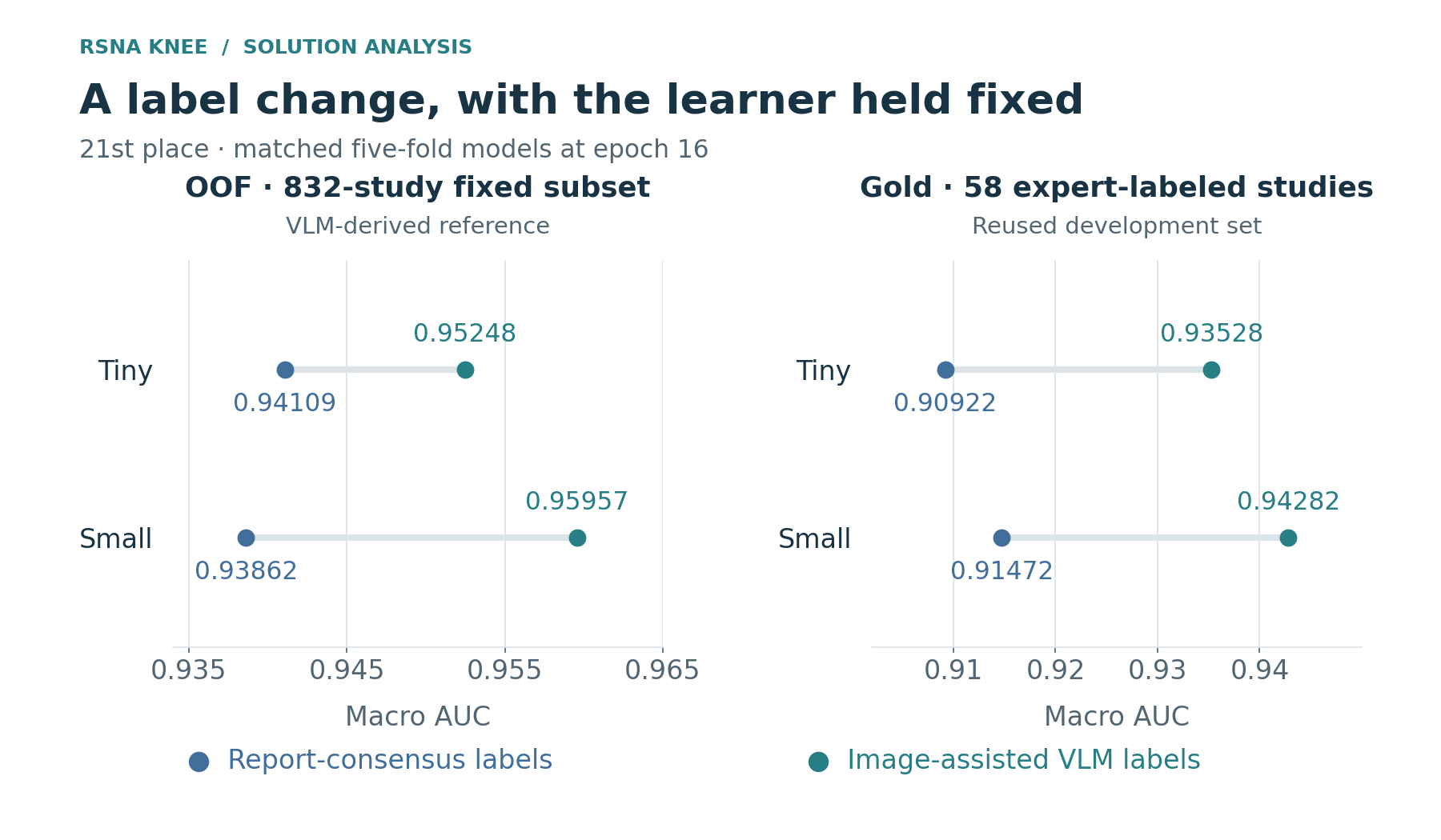
Figure 1. The 21st-place fixed-epoch comparison. OOF uses 832 predefined random studies and image-assisted probabilities above 0.5 as positives; gold uses 58 expert cases reused in development. Panel scales differ.

Student and training target	832-study OOF AUC	Expert-58 AUC
ConvNeXt-Tiny, report consensus	0.94109	0.90922
ConvNeXt-Tiny, image-assisted	0.95248	0.93528
ConvNeXt-Small, report consensus	0.93862	0.91472
ConvNeXt-Small, image-assisted	0.95957	0.94282

The large reference set shares the new label lineage, so its improvement alone cannot establish closer agreement with expert targets. Improvement in the same direction on the expert cases supplied a second reason to continue the annotation campaign, although those repeatedly inspected 58 studies were not an independent clinical test. Both columns evaluate trained students; neither is simply the AUC of the source label table.

My H1c experiment already followed part of this logic. The image-assisted reader saw up to twelve fluid-sensitive slices, four per plane, with the report. The pilot included report-only comparisons, repeated readings, and images replaced by those of another study: 275 calls across the designed controls. A hundred pilot cases were reused, and 4,307 additional cases completed coverage of 4,407 studies. I trained matched complete five-fold mmE and mm12 students and kept the clean baseline identity. In that small-student setting, mm12’s Public AUC was 0.914 against 0.911 for the control.

The pilot nevertheless exposed a coverage problem: four images per plane could miss localized marrow findings. Effusion responded to correct images and to image substitution, whereas contusion remained strongly report-dependent. A wrong-image control could establish visual influence or expose report anchoring; it could not establish that the answer was grounded in the correct lesion.

The unresolved question was whether better access to the relevant anatomy, or a stronger reader using that access, could produce targets that the same student learned more effectively.

Reader diversity and the cost of better evidence

Several lower-ranked accounts help distinguish a new information source from another pass over the same text. The forty-ninth-place author averaged local Qwen readers and public labels to reach about 0.895 label AUC, then added a hosted descriptive reader to reach 0.899. It also reported a five-level rubric response at only 0.809, below the public regex baseline, because quantized outputs collapsed useful ranking distinctions. A schema separating mention, severity, and code-assigned probability was more effective. That is an output-representation failure, not evidence that medical definitions were unimportant.¹⁶

The 102nd-place author generated twenty responses per study: five original-language and five translated-report responses for each of two local models. The source then used explicit rules linking unmentioned synovitis to effusion and OA. This was a substantial ensemble of report interpretations, but all responses still depended on the same original text and assumptions about missing findings. The seventy-second-place author likewise found no Public gain from adding more report-reader sources, despite reasonable label AUC and varied model names.¹⁷¹⁸

Diversity could still help. In sakaku’s final Mix5, Astra v1, Astra v2, a teammate’s Astra source, Hulu, and Qwen contributed 30%, 20%, 30%, 10%, and 10%, using the same weights for every finding. An earlier attempt at flexible target-specific fusion lost its apparent advantage under leave-one-out evaluation. The result was a small mixture of distinct readouts with fewer fitted choices, not proof that one particular provider or a growing list of readers was indispensable.

Annotation economics also differ from training economics. A twenty-one-image packet, a 277-image request, and a viewer session have different token, caching, latency, failure, and coverage costs. A full programme needs the reader or subscription capacity, image rendering, storage of source identities, accepted-case resumption, probability checks, student training, and delivery into the final inference system. Sakaku recorded cached input, uncached input, and output separately and resumed only unfinished cases. The twenty-first-place author reported completing its remote-viewer annotation without extra API or subscription-quota spending in that setup; this is a reported access arrangement, not a universal zero-cost estimate.

Across these accounts, supervision quality depended on what the reader could inspect, how its evidence became a target, and what the student could learn from that target. Better annotation could strengthen a classifier without adding a test-time model. Its value still depended on the student’s image representation: a target can describe a lesion that the student’s crop or sampling has removed.

2. Image information and model structure

Physical geometry and information coverage

An MRI study is a collection of spatial measurements, not a fixed number of interchangeable pictures. The same array size can represent different fields of view; the same number of slices can cover different depths; adjacent array entries can be separated by different distances. A classifier can only learn from the evidence its preprocessing preserves. Increasing backbone capacity cannot reconstruct a meniscal edge that was discarded before the forward pass.

For an in-plane field of view $F$ millimetres resized to $N$ pixels, the nominal scale is $F/N$ millimetres per pixel. The fifth-place system used 150 mm full-field images at 384 pixels and 80 mm regional crops at the same size. Those correspond to approximately 0.39 and 0.21 mm/pixel. A 2 mm structure occupies about 5.1 pixels in the former and 9.6 in the latter. This is nearly 1.9 times the linear sampling density, although interpolation cannot create detail beyond the original acquisition. The benefit is avoiding the loss of available local detail when compressing the whole knee into the input grid.¹

Depth matters as much as in-plane scale. Sorting filenames or instance numbers is not a substitute for sorting physical slice locations. If $P_k$ is a slice’s patient-coordinate origin and $n$ its plane normal, the scalar $n^\top P_k$ supplies its position along the stack. In-plane axes and pixel spacing then map a pixel to a patient-space location. A crop, a lesion annotation, and the corresponding view from another sequence must use compatible transforms. Otherwise, a perfectly functioning tensor pipeline can connect a label to the wrong anatomy.

This also clarifies the ambiguity in “three-slice input.” Three consecutive original slices retain the acquisition’s local depth sampling. Three neighbors after selecting 32 evenly spaced positions from a series span a different physical distance. The 32nd-place team specifically used truly adjacent original DICOM slices; the winning team’s sakaku branch formed triplets from 32 sampled positions, which need not be consecutive source slices. Neither description is wrong, but they define different inputs. The relevant question is whether the resulting slab can show the structure and depth context needed for the target.⁹⁸

My native-field N path retained a 0.4 mm/pixel representation up to a 204.8 mm field and aggregated thin source slices into approximately 3.5 mm slabs. S6F combined full-field views with local views anchored by the SKM-TEA localization model. The remaining coverage questions were finding-specific: whether a crop retained the superior fluid pocket, whether a lateral-compartment view cut off the relevant meniscal edge, and whether selected positions skipped a thin lesion.

Wider coverage can reduce sampling density. The 977th-place author widened the span to the central 2–98% while retaining 44 slices, and the reported score fell from 0.926 to 0.917. Increasing to 64 slices within that wider span reached 0.928. The source does not identify the metric as Private. This comparison tests span and density together: more anatomy entered the input, but enough sampled positions were needed to preserve its local detail.¹⁹

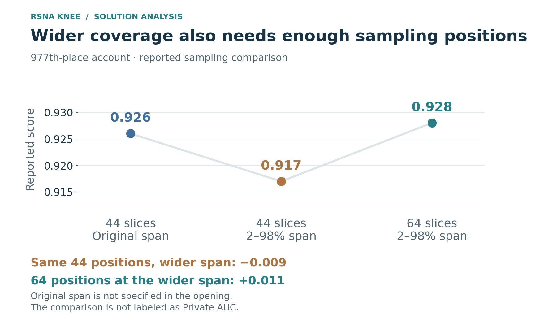
Figure 2. The 977th-place account reports 0.926 for the earlier 44-slice recipe, 0.917 after widening to 2–98% at 44 slices, and 0.928 at 64 slices with the wider span. The earlier physical span is unspecified and the quoted score is not identified as Private.

The second-place team found an input bug that made early models read only four pictures per series. Reading fifteen improved its 58-case development AUC by 0.033. That number is not a Private gain and does not isolate every possible effect of increased sampling, but it explains why the authors ranked the correction above most architecture changes. The 74th-place author similarly reported that an early fixed-count sampler lost about 28% of slices, disproportionately from long series, and moved to reading all slices. Those examples make input coverage a scientific variable rather than a housekeeping detail.³¹¹

Sequence roles, laterality, and missing views

Even correct geometry does not tell the model what contrast it is reading. Fat-suppressed fluid-sensitive images, structural views, and different planes expose different aspects of a finding. Pooling them as an unordered stack asks the network to infer these roles from appearance while also learning the disease target. Reliable role metadata can remove part of that burden, provided the metadata is itself checked.

The 22nd-place solution devoted substantial effort to that check. Its audit covered 24,371 series. Of these, 13,046 lacked a usable description, and examples with apparently informative names included rescans and reconstructions whose name no longer matched their contents. The final rules combined the host table and DICOM acquisition fields: plane, inversion recovery, gradient-echo status, repetition and echo times, fat-suppression hints, obliquity, and 2D/3D information. PD and T2 were not split by an arbitrary name boundary; echo time was also available to the model as a quantity. Only the subset missing sequence, TR, and TE required a name-based weighting fallback.⁷

A subtle example was the host’s Fat_Suppression flag: the author interpreted its operational meaning as fluid-brightness rather than a complete physical description of all fat-suppressed sequences. Water-selective acquisitions and inversion-recovery images needed additional rules. Feeding a categorical “FS” token without understanding its derivation could therefore communicate a different property than intended. Conversely, indiscriminately adding scanner, coil, sex, and site-identifying metadata could strengthen report prediction through a site-related shortcut.

Laterality normalization had a related purpose. Most targets distinguish medial from lateral anatomy, not the patient’s left knee from the right. Putting both sides into one anatomical convention reduces a nuisance transformation. However, an image-width flip does not mean the same physical operation in every plane. The 977th-place author used channel reversal for sagittal triplets and width reflection for coronal and axial windows. The 32nd-place team aligned sagittal position embeddings under anatomical mirror TTA. In both cases, location and input transformation had to describe the same anatomy.¹⁹⁹

The 22nd-place side pipeline used tags, image position, and then a small image classifier to resolve conflicting evidence. Series selection retained useful oblique coronal acquisitions near the ACL rather than rejecting obliquity categorically. It deduplicated repeated acquisitions by their attributes, favored new sequence types in available slots, and filled empty slots from the remaining series. Three-slice windows never crossed a series boundary. Each rule changed the anatomy or contrast that the model actually received.

Missing input also has more than one meaning. A role can be absent because the scan lacks that acquisition, because selection failed, or because decoding failed. Masking a missing role is different from silently filling it with another contrast. Sakaku’s model explicitly represented valid and non-repeated slices and masked missing roles. The 22nd-place author reported that several inference-time substitutions for an unusual weak-effusion group did not help; attribute-aware input later recovered only part of its deficit. A missing-view problem cannot always be repaired by finding any tensor of the expected shape.⁸⁷

Window bags and finding-specific aggregation

A study contains many possible image windows and only twelve study-level targets. Multiple-instance learning provides a practical bridge. A shared 2D encoder produces a feature for each window; an aggregation head decides which windows contribute to each finding. This retains pretrained 2D backbones without requiring a complete 3D volume at every step.

A common finding-specific attention model has window feature $h_j$, score $s_{c,j}=w_c^\top\tanh(Vh_j)$, and pooled representation

\[\beta_{c,j}=\frac{\exp(s_{c,j})}{\sum_k\exp(s_{c,k})},\qquad r_c=\sum_j\beta_{c,j}h_j.\]

Separate $\beta_{c,j}$ lets an ACL prediction and an effusion prediction use different evidence. Hierarchical variants first pool windows within a series and then pool series within the study. Spatial variants also select positions within the backbone feature map. These are different levels of the same information-allocation problem; adding the name “MIL” does not identify which bottleneck has been addressed.

The seventh-place model made position explicit. A shared CNN converted each window into a grid of tokens. The tokens carried series identity and 3D coordinates in a common knee frame; crop affines were used to map local coordinates back to that frame. Two queries per finding attended over tokens, while a gated MIL head supplied another readout. Their logits were averaged. Thirteen fixed regional zoom views supplemented the full series, so the decoder could compare fine local evidence with broader context.⁴

Its train–test bag sizes differed substantially. Inference evaluated a window at every slice of each retained series and zoom region. The author sharpened attention for the larger bag, using multipliers of 1.75 for EfficientNetV2-S and 1.25 for ConvNeXt. A simplified example explains the concern: if one informative token has score $a$ and $K-1$ irrelevant tokens have score $b$, its attention mass at sharpness $\tau$ is

\[\frac{1}{1+(K-1)\exp[-\tau(a-b)]}.\]

Increasing the bag while retaining the same score separation can dilute the informative token. Sharpening may offset that dilution, but it can also amplify a spurious maximum. The multipliers were choices for this recipe, not universal settings for dense MRI inference.

The 22nd-place model added a two-layer window Transformer before attention pooling. Its residual output projection began at zero, so the initial network behaved like the simpler pooling model; the author reported collapse without that initialization. Window tokens received plane, position, and acquisition embeddings, and acquisition attributes were sometimes hidden during training. These details illustrate a more useful architecture question than “Transformer or CNN”: how to add communication between windows without destroying an already useful initialization.⁷

S6F already had finding-specific spatial and window attention. The remaining questions concerned what its tokens preserved, whether the head could identify their physical role and location, and whether direct supervision made a high-attention position meaningful. Replacing the head alone could leave predictions highly correlated when the input and supervision remained unchanged.

Anatomy regions and lesion evidence

An anatomy ROI answers “where should this finding be assessed?” A lesion box answers “where is visible abnormal evidence?” A normal meniscus still has an anatomy ROI, and an unannotated lesion is not automatically absent. The winning team’s two branches made this distinction useful in different ways.

Tascj’s branch restricted pooling to a finding-specific 3D ROI. With feature vector $v_r$, cell-overlap weight $o_{c,r}$, and learned score $a_{c,r}$, its normalized attention has the form

\[\alpha_{c,r}=\frac{o_{c,r}\exp(a_{c,r})}{\sum_j o_{c,j}\exp(a_{c,j})}, \qquad h_c=\sum_r\alpha_{c,r}v_r.\]

Here the normalization spans the relevant series’ cells and slices, not just a single image. The archived implementation estimates overlap by subcell sampling and masks the ROI’s depth extent. It requires positive overlap mass; an empty ROI falls back to a series mean. Starting the attention convolution at zero makes the initial operation an overlap-weighted average. The model learns which evidence matters within a prescribed region rather than discovering both location and diagnosis entirely from study labels.²⁰

The same branch used lesion coverage and report-embedding auxiliary heads. The code’s annotation-state mask excludes unavailable supervision, and the inference loader removes the auxiliary head weights. However, its ROI detector and side classifier still run at test time. Removing a training loss does not remove the cost of finding the input region.

Sakaku’s branch instead used spatial annotation mainly to teach a shared feature extractor. Six targets—MCL, both menisci, and the three OA compartments—combined a global feature $g$ with an anatomy-attended feature $a_c$ through

\[h_c=g+\gamma(a_c-g),\qquad \gamma_{\mathrm{init}}=0.1.\]

The residual begins close to global pooling and can learn how much local evidence to use. Regional MIL, attention-mass constraints, and reliable-negative window supervision guided the attention. The other six targets retained global spatial pooling. This does not assume that every finding should be localized to a small region; it gives the anatomy-specific targets a route to use location without discarding general context.⁸

A twelve-target lesion-evidence head reused the same backbone map. Its pooled evidence contributed a prevalence-centered residual, reported as $z=z_{\mathrm{main}}+0.25(e_{\mathrm{lesion}}-\operatorname{logit}\pi_{\mathrm{train}})$. The prevalence term used the training data. This subtracts a prior term from the added evidence route; it does not establish that the resulting logit is clinically calibrated.

Annotation alignment was central. The lesion archive covered requested findings on identified series and slices. Supervision required compatible geometry, the valid central slice of a triplet, and eligibility rules. A missing requested record, an invisible lesion, and an explicitly negative finding were not collapsed into one state. In a generic masked spatial objective,

\[\mathcal L_{\mathrm{spatial}} =\frac{\sum_{i,c,r}m_{i,c,r}\,\ell(\hat e_{i,c,r},a_{i,c,r})} {\sum_{i,c,r}m_{i,c,r}},\]

$m$ indicates eligible supervision, not lesion presence. The loss is evaluated only when that denominator is positive. Replacing every missing annotation by a negative changes the learning problem from locating evidence to copying the annotation procedure’s misses.

This branch needed no annotation files or detector pass at test time. Its image feature map had already been computed for classification, so local supervision strengthened a readout without another backbone pass for every crop. An earlier half-image meniscus route cost roughly 2.2 times the backbone evaluation; feature reuse offered a different performance–cost tradeoff. The complete anatomy-aware package improved Public 0.956 to 0.960, while its local difference was inconclusive. Multiple components changed, so the score belongs to the package rather than one isolated loss.⁸

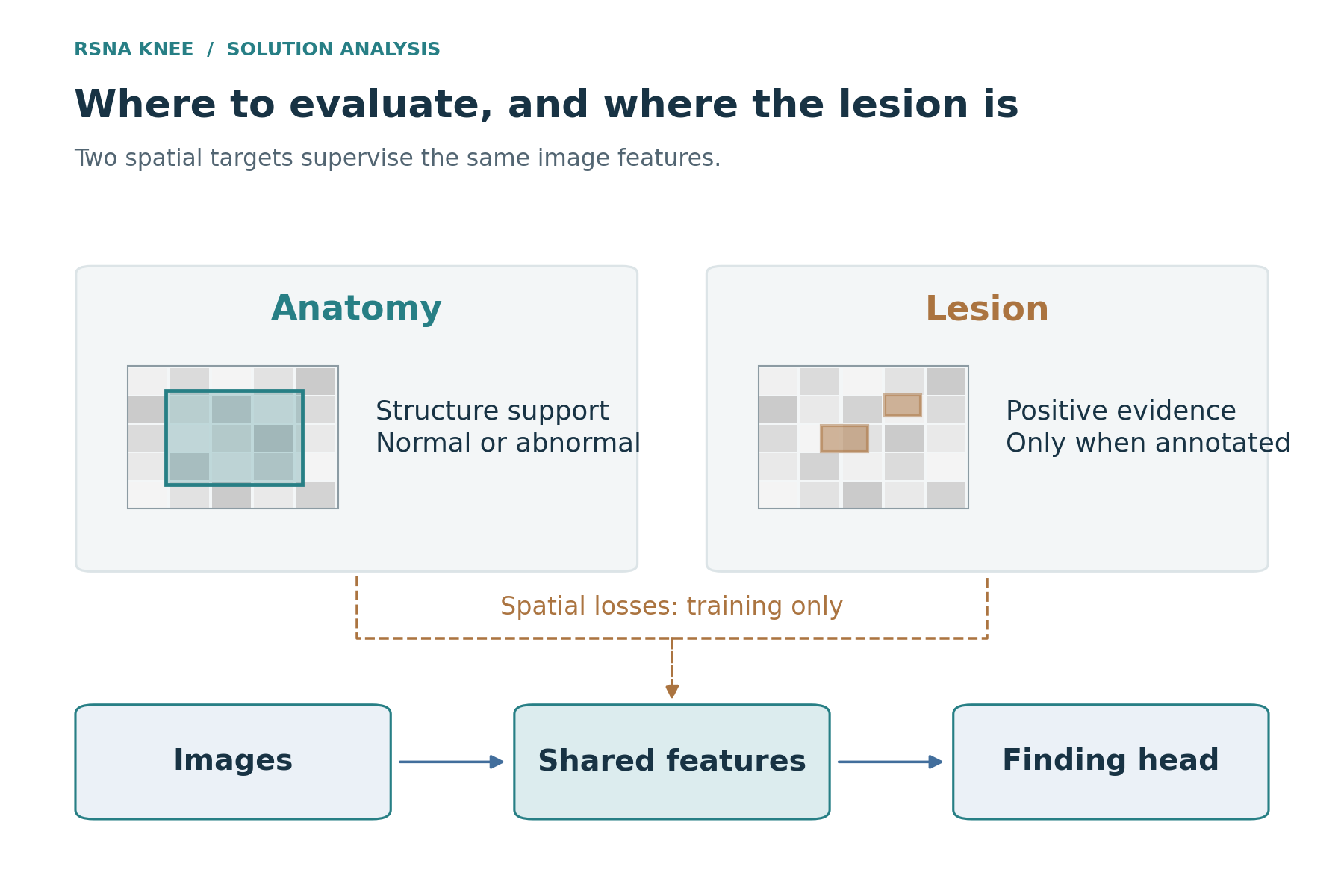
Figure 3. Anatomy ROI guides where to look; lesion evidence supplies spatial targets; unavailable annotations are masked. Training-only spatial losses reuse classifier features. A detector-assisted inference route has an additional test-time cost.

Tascj also used six-channel variants for complementary views. These were not six adjacent slices. The channels represented fixed plane-by-fat-suppression roles, resampled in patient coordinates onto the current series. That changes which contrasts enter one encoder evaluation. Resampling establishes a coordinate convention, but cross-sequence anatomy can still differ because of positioning and motion; the protocol is more specific than simply concatenating six arbitrary images. The author reported more benefit from this view change than from backbone diversity alone.²⁰

The winning output combined this three-model branch with tascj’s branch at 1:1. Tascj’s five run groups contain 17 classification checkpoints; sakaku contributed three full-data models. The archived integration confirms the branch weighting. These are not twenty equally weighted models, nor evidence that a particular model count is optimal.²¹

Compartments, context, and targeted specialists

The fifth-place system located four crop regions from femur, tibia, and patella masks. Its nnU-Net was initialized from TotalSegmentator-MRI and trained on 1,200 competition series. Regional crops entered as additional tagged series, increasing the average input from about 5.5 series to 17.6. Bone segmentation and laterality classification also ran at test time, so the gain in spatial detail came with additional preprocessing and image evaluation.¹

Its score progression separates two useful steps. EfficientNetV2-M with newer labels and longer training reached Private 0.954; adding anatomy-guided crops with the same model and labels reached 0.957. ConvNeXt-B with those crops reached 0.958. The earlier 0.946 to 0.954 step changed labels and epochs together; the crop step is the more direct input comparison. The final ensemble remained at 0.958, showing that a strong regional basis had already captured much of what later additions supplied.

Input intervention	Concrete mechanism	Reported limitation
Second-place detail plus context	Knee-centered close-up and whole-knee evidence	Close-up alone lost 0.010 on Lateral Meniscus before context was restored
Fifth-place regional crops	More pixels on joint and compartment structures	Specialists added at most about 0.001 on the stronger regional basis
Twenty-second-place compartment input	One compartment at a time, shared weights	Post-hoc medial/lateral subtraction instead lost 0.007 Public
Thirty-second-place attention-guided zoom	Select windows, reread original pixels at roughly 2× zoom	Extra findings or 30% rather than 20% zoom weight hurt

The second-place close-up-only model lost 0.010 on Lateral Meniscus until whole-knee context was restored. Local detail and context had to complement each other. The pinned public rewrite estimates the knee centre from geometry and tissue width, then combines separate detail/context pooling through a gate. It supplied a concrete localization method without requiring a new large segmentation training project.³²²

The 22nd-place solution attacked a different error: predicting lateral OA from correlated medial degeneration. Its shared-weight compartment model sees one compartment at a time; lateral inputs are mirrored into the same convention. The model cannot directly inspect the opposite compartment. Its fourth compartment classifier also changed the labels of certain discordant negatives and moved the crop to the weight-bearing zone. That model carried 74% of the final lateral OA weight. The intervention combined restricted information, consistent anatomy, and altered supervision—not simply a larger network.⁷

The 32nd-place zoom model selected six window groups per difficult target, returned to the original DICOMs, and extracted higher-resolution lateral-compartment or patellofemoral views. The selector itself belonged to each fold’s training pipeline. The student used the held-out fold only for evaluation; a selector trained on those cases would have compromised the comparison. Zoom entered only Lateral Meniscus, Lateral OA, and PF OA. Increasing its contribution or extending it to other findings was harmful.⁹

The fifth-place team likewise checked actual missed evidence. Its earlier bone crop retained only 78–80% of the slices cited for effusion and synovitis; the omitted slices were above the crop. Extending the axial slab upward by 20 mm addressed a concrete coverage defect. Of forty short weak-finding fine-tunes, only Lateral Meniscus passed its checks. That fine-tune reused the main model’s earlier layers. These choices make “specialist” precise: a targeted error and a targeted computational addition, not another full model added because the budget still has room.

The 73rd-place KneeSplatNet experiment is a useful test of how much those additions actually establish. It mapped each stride-16 feature cell into a common knee frame and splatted features into a 12 × 12 × 12 grid at 8 mm spacing. Separate fat-suppressed and other banks, anatomical anchors, hit masks, and a medial–lateral difference volume supplied a coarse 3D representation alongside ordinary 2.5D pooling. This was a concrete geometric model rather than a generic extra attention block.²³

The author then disabled components at inference on the same checkpoint, evaluating 477 held-out studies from two folds against LLM-derived references. Removing the 3D path cost 0.0049 macro AUC, removing geometry cost 0.0011, and removing the earlier-stage projection cost 0.0021. Those knockouts demonstrate that the trained network used the components. They do not establish that adding them was better than training the matched simpler model: the complete KneeSplatNet did not beat its 2.5D control overall. It moved accuracy toward the anterior compartment and PF OA while giving up performance on ACL, menisci, and contusion.

The final predictor instead combined 2.5D ConvNeXt-Tiny models with a patellofemoral close-up model. The 3D-splat prototype’s component knockouts showed what the fitted network used; the matched simpler control showed whether that use improved overall performance. Its finding-specific gains could still motivate a specialist or complementary arm, but the prototype was not a demonstrated final improvement.

Pretraining and the use of external MRI

External MRI did not play one uniform role. It could initialize anatomy, teach a task-specific encoder, supply independent grading, or add partially supervised training rows. Those choices expose different domain and target mismatches.

The second-place mil-reader used fastMRI knee images and fastMRI+ boxes for pretraining. Its PF specialist added a head trained on OAI cartilage grades. The fifth-place backbones first predicted 327 binary readings derived from MOAKS/WORMS grades on 2,414 OAI knees; two single-model tests reported about +0.001 Public from that start. Such results support particular uses of external information rather than the claim that adding outside cases is inherently advantageous.³¹

The 63rd-place author reported a useful contrast. Three epochs of DINO pretraining used roughly 371,000 competition triplets and 380,000 fastMRI triplets. Without fastMRI, the pretraining was flat; including it improved OOF by 0.003 and an external OAI check by 0.006. Yet six experiments using OAI MOAKS as additional supervision were negative, with two principal fold-0 variants down 0.010 and 0.013. For that system, images helped through self-supervised representation learning while the tested partial-label supervision did not.²⁴

The 977th-place system added 5,178 OAI knees whose supervision came from radiographic joint-space grading, contributing only to medial and lateral OA cells. Its local macro AUC fell 0.9277 to 0.9161; lateral OA fell 0.807 to 0.774. The author’s proposed explanations were modality/definition mismatch and changed gradient allocation when many external rows supervised only two findings. Those observations do not prove which explanation dominated, but they show why a larger training set need not teach the desired MRI target.¹⁹

The 74th-place solution used OAI readers more selectively, to reorder labels or vote on findings for which the external model transferred acceptably. Medial meniscus and medial OA were rejected for label correction because their coupling looked wrong on other evidence. The 32nd-place OAI branch was weaker alone on Public, 0.960 versus 0.961, but helped its main mixture. The contribution was a change in errors, not a mandatory standalone win.¹¹⁹

These examples separate four uses of external MRI: additional training images, useful initialization, a mapped disease head, and an external diagnostic panel. “Acquire OAI” leaves the experiment unspecified. Modality, finding definition, missing-label treatment, fold ancestry, and the route into the final prediction determine which use is being tested.

Optimization trajectories and pretrained adaptation

A strong label source still has to be absorbed by the learner. Sakaku reported increasing the backbone peak learning rate from $8\times10^{-6}$ to $8.944\times10^{-5}$ in an earlier 224-pixel CoAt comparison. Public rose 0.936 to 0.944, while the 58-case development AUC fell 0.9283 to 0.9215. The intervention also changed how long training continued under its stopping rule. It therefore supports a better learning trajectory under that intervention, not a clean numerical decomposition of learning-rate and duration effects.⁸

The final three models trained for nineteen epochs on the original thirty-epoch OneCycle horizon, then averaged EMA checkpoints from epochs 15–19. A nineteen-epoch fit on that schedule is not equivalent to compressing the full decay into nineteen epochs. The learning-rate values seen at each update, and the checkpoints being averaged, differ. Reproducibility needs the schedule horizon as well as the stop epoch.

Other solutions reinforce the distinction. The seventh-place ConvNeXt models used a thirty-epoch schedule stopped at epoch twenty, with late weight averaging. The fifth-place newer-label comparison also increased training from seventeen to twenty-five epochs. The 22nd-place author accepted nothing on a mid-training score and averaged late weights; its residual Transformer needed an initialization that preserved the initial pooling model. Successful recipes paid attention to optimization behavior rather than treating a short checkpoint as an architecture verdict.⁴¹⁷

Longer or larger was not automatically better. Larger decoders, slice mixers, heavier augmentation, and larger backbones repeatedly failed in the seventh-place experiments; the 63rd-place author found no gain for the cost from several larger alternatives. The distinct hypotheses were a lack of representation capacity, inadequate input, and insufficient adaptation of existing features. A short architecture swap could not distinguish them by itself.

Shared computation and the meaning of a runtime result

Inference cost includes decoding, geometry and ROI preparation, backbone evaluation, aggregation heads, transfer, startup, and slow-case tails. Some of those stages can overlap, and some can be shared between members. Summing isolated notebook times assumes neither. Counting only checkpoint FLOPs ignores both.

For a simplified stream of $N$ comparable studies, CPU preparation time $t_C$, GPU time $t_G$, $W_C$ preparation workers, and $W_G$ GPU workers, an overlapped pipeline approaches

\[T\approx T_{\mathrm{startup}} +\max\!\left(\frac{Nt_C}{W_C},\frac{Nt_G}{W_G}\right) +T_{\mathrm{tail}}.\]

This is a throughput model, not a hidden-test forecast. Studies have different numbers of series and windows; file access and crop failures create tails. It explains why accelerating the backbone may achieve little when decoding is the bottleneck, and why sharing one decoded study across compatible models can be more valuable than removing a small head.

The fifth-place implementation decoded and placed crops once for M1–M3, reused early M3 features for its Lateral Meniscus fine-tunes, and ran one process per T4. The 22nd-place system shared decoded DICOMs and overlapped segmentation/cropping with model inference. Its 56 networks fit, while 61 did not always. Those are complete-system engineering claims, not a conversion rule from network count to hours.¹⁷

The first-place efficiency route used a different operating point: 256-pixel input, a single full-data checkpoint, fluid-sensitive selection, C++ DICOM handling, FP16 TensorRT, and 230 seconds on a 1,200-study benchmark constructed from training data. This is valuable evidence that substantial processing overhead could be removed. It is not the runtime of the full 384-pixel winning ensemble on the hidden test.²⁵

Termination policy also changes what a reported runtime means. The second-place kernel writes core predictions first and adds specialists that finish within their budgets; unreadable studies receive defaults. The seventh-place notebook can retain neutral ranks for failed cases. The fifth-place pipeline budgets stages, and the 22nd drops failed models and renormalizes weights. My declared policy was to compute the entire specified composition or fail, without silently shrinking members, windows, or series. I can reuse their decode-sharing and efficient batching without treating their dynamic fallback results as proof that my exact complete composition fits.

An inference result therefore needs both an exact operator and an execution policy. A sample pass verifies the visible cases, a component estimate prices a proposed route, and a complete run tests feasibility on the actual workload. Efficiently computing a view still leaves a separate question: whether that view teaches the classifier the intended finding or a correlate of how it was reported.

3. Reporting effects, validation, and distillation

Report-site effects and the observation model

Report-derived targets reflected more than image findings. A radiologist’s threshold for mentioning cartilage loss, fluid, or synovitis could depend on local practice, while acquisition differences made the source institution recognizable from the MRI. Recognizing the site could therefore improve prediction of the training reference without improving recognition of the finding. Patient-group separation prevents memorization of the same patient, but not a reporting shortcut shared by other patients at the same institution.

The 38th-place solution measured report-positive rates ranging from 4.6% to 30.3% for lateral OA, 10.0% to 43.7% for PF OA, and 0.5% to 13.7% for synovitis across report languages. Its image model’s mean predictions correlated with the language-level report rates at 0.99 for lateral OA and 0.96 for medial OA. Acquisition metadata predicted report language with 98% accuracy in the 33rd-place analysis, compared with a majority-class baseline of 39%. These observations do not prove that the prevalence differences were spurious. They establish that an image model had access to a plausible proxy for the reporting process.¹⁵²⁶

For a simplified model of that process, let $Y$ denote an expert-defined finding, $R$ whether a report records it, $X$ the MRI, and $S$ the site. Define

\[a_s=\Pr(R=1\mid Y=0,S=s),\qquad b_s=\Pr(R=1\mid Y=1,S=s).\]

Under the assumption $R\perp X\mid(Y,S)$, and writing $\eta(x,s)=\Pr(Y=1\mid X=x,S=s)$,

\[\mathbb E[R\mid X=x,S=s] =a_s+(b_s-a_s)\eta(x,s).\]

When $b_s>a_s$, report probability preserves disease ordering within a site. Site-specific offsets and sensitivities can nevertheless reverse the order of cases from different sites. Assume two cases have disease probabilities 0.70 and 0.40. Reporting parameters $(a,b)=(0.05,0.55)$ and $(0.20,0.95)$ give report probabilities 0.40 and 0.50: reporting is informative within each site, yet the report target reverses the clinical order across them.

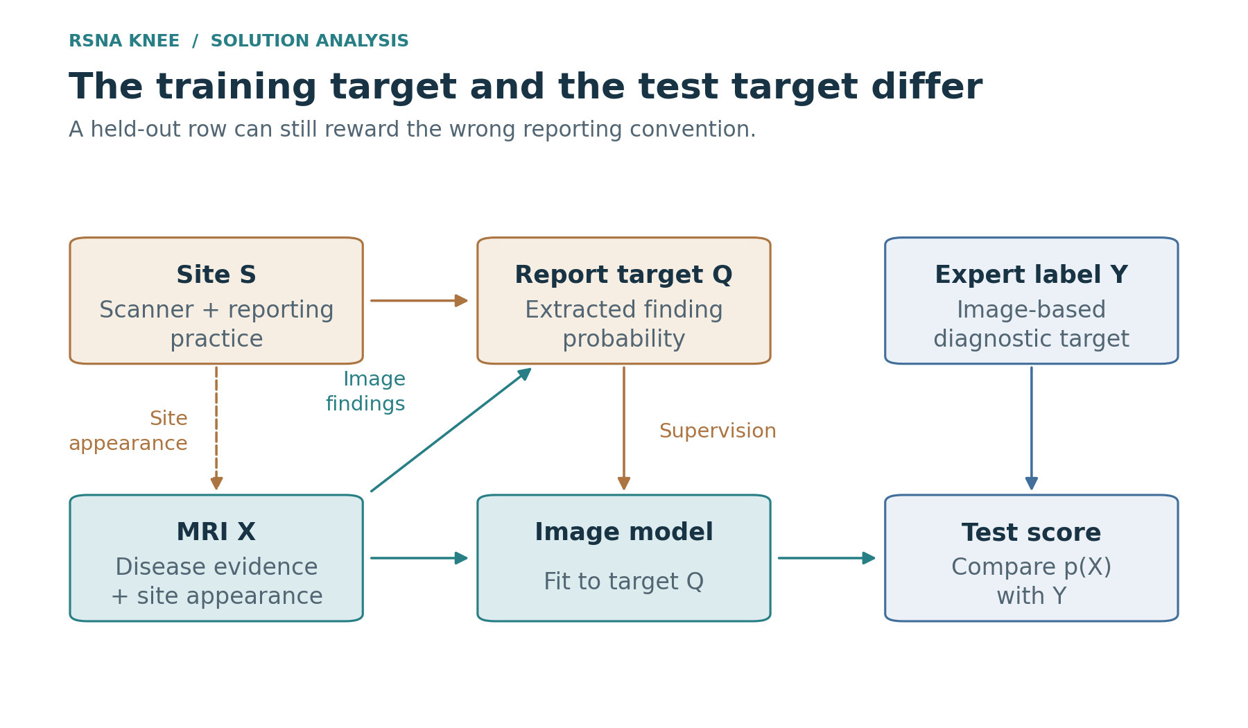
Figure 4. The report target receives clinical image evidence and site-dependent reporting effects. Site also affects acquisition appearance and genuine case mix; a fold split does not isolate these mechanisms.

The actual targets were soft probabilities extracted from reports, not binary $R$. Nevertheless, their training objective could reward the same mixture of disease evidence and reporting convention. For unweighted expected BCE, an unrestricted population minimizer predicts $\mathbb E[Q\mid X=x]$, where $Q$ is the constructed target. No fold assignment changes which conditional expectation the loss asks the learner to approximate.

The training-only site terms used by the 33rd, 38th, and 72nd teams gave the reporting component another route through the loss:

\[\mathcal L=\sum_{i,c}w_{i,c}\, \ell_{\mathrm{BCE}}\!\left(q_{i,c}, \sigma\!\left(f_c(x_i)+u_{s_i,c}+g_c(m_i)\right)\right).\]

Here $u$ is a site table, $m_i$ acquisition metadata, and $g$ an optional metadata branch. At inference the teams retained only the image logit $f_c(x)$. The equation summarizes their common design; the 72nd-place model used the site table without the 33rd-place acquisition MLP. These branches gave reporting patterns a separate path through the training loss, reducing the need for the retained image path to represent them. That does not make $f$ site-invariant: the image network can still recognize the site, and removing every site difference could also discard real case-mix information.

Interventions that separated reporting habit from disease evidence

The strongest evidence came from interventions rather than the geographic variation alone. The 33rd-place author first found that turning off acquisition-dependent components at inference, with the same checkpoint, improved Public/Private from 0.947/0.929 to 0.959/0.944. This avoided training-seed variation in that comparison. It suggested that the component intended to exploit acquisition information was reproducing a property that the expert test labels did not reward.²⁶

The later controlled training progression was distinct:

OrthoFoundation-L recipe	Public	Private
No acquisition inputs or trap	0.949	0.932
Site term	0.955	0.940
Acquisition branch and empirical-Bayes initialization	0.960	0.946
Teacher-spread targets for unmentioned findings	0.962	0.947

The site term was regularized as a random effect, and the acquisition MLP had a zero-initialized output. Because the final row also changes the targets, the full progression combines site modeling and target reconstruction. The author also applied the recipe to a CoAtNet backbone and reported 0.961/0.948.

The 38th-place account added a useful reversal check. With its main labels and the same recipe and seed, a language-based training offset moved 0.949/0.935 to 0.953/0.938. Adding the learned offset back at test, using a metadata-predicted site, reduced the same checkpoint to 0.950/0.936. A finer 29-site key subsequently reached 0.955/0.941. These are separate comparisons: initial offset, restoration, and site refinement. Their value lies in testing the proposed direction, not in adding three gains together.¹⁵

The 72nd-place author repeated the intervention at two resolutions:

Student input	Without site bias, Public/Private	With site bias, Public/Private
288 pixels	0.947 / 0.932	0.953 / 0.939
384 pixels	0.948 / 0.933	0.954 / 0.940

Both Private differences were +0.007. Retraining its label teachers with site bias then produced 0.955/0.942; that later result is a new target-generation intervention, not the score of the original site-only ablation.¹⁸

Other teams changed the targets or final predictions instead of the training logit. The 63rd-place solution partly rank-mapped each site cluster onto the pooled target distribution. Its site-cluster step moved a three-model bundle from 0.955/0.942 to 0.957/0.947. Full mapping was worse than partial mapping: gold AUC fell from 0.9371 to 0.9268 at mapping strength 1.0. Equalizing distributions had erased useful differences as well as nuisance differences.²⁴

The 228th-place author trained metadata-only report predictors and subtracted a small part of their rank from a public blend. Adding that prior first made Public worse, supplying a sign check. Early debiasing improved Private 0.942 to 0.945; the later Public-best refinement scored 0.944. The 246th-place solution instead reduced excessive coupling between OA compartments. Its correction lost on report-reference OOF in all nine tested reader–member cells while an external expert panel supported the opposite direction.²⁷²⁸

A label-distribution correction, a training-only nuisance branch, and a final rank subtraction intervene at different points in the pipeline. Their results show why a local/Public disagreement needs a diagnosis: the learner may be improving at predicting the reporting process rather than the expert finding.

Pooled AUC, within-site AUC, and the reference being predicted

For a fixed binary reference $Z$, pooled AUC can be decomposed into comparisons between sites:

\[\operatorname{AUC}_{\mathrm{pooled}} =\sum_{s,t}\pi_s^+\pi_t^-A_{s,t},\]

where $\pi_s^+=\Pr(S=s\mid Z=1)$, $\pi_t^-=\Pr(S=t\mid Z=0)$, and $A_{s,t}$ scores a reference-positive case from site $s$ against a reference-negative case from site $t$. Ties receive half credit. When $Z$ is a report-derived reference, these are report-positive and report-negative groups—not the unknown expert groups.

Pooled AUC rewards both within-site ordering and cross-site offsets. Mean within-site AUC removes the $s\ne t$ comparisons and then applies a chosen weighting over sites. It therefore changes the question. A model that correctly identifies high-prevalence clinical populations could lose under that restriction, while a model exploiting a reporting convention could lose for the right reason. Neither score identifies which explanation applies on its own.

In the 72nd-place study, adding site bias reduced pooled report-reference OOF 0.912 → 0.906, while mean within-site OOF was nearly unchanged, 0.906 → 0.907. Public improved by 0.006 and Private, revealed later, by 0.007. Across 26 single models, the author later measured Spearman correlations with Private of −0.83 for pooled report OOF, +0.56 for within-site OOF, +0.78 for gold-58, and +0.94 for Public.¹⁸

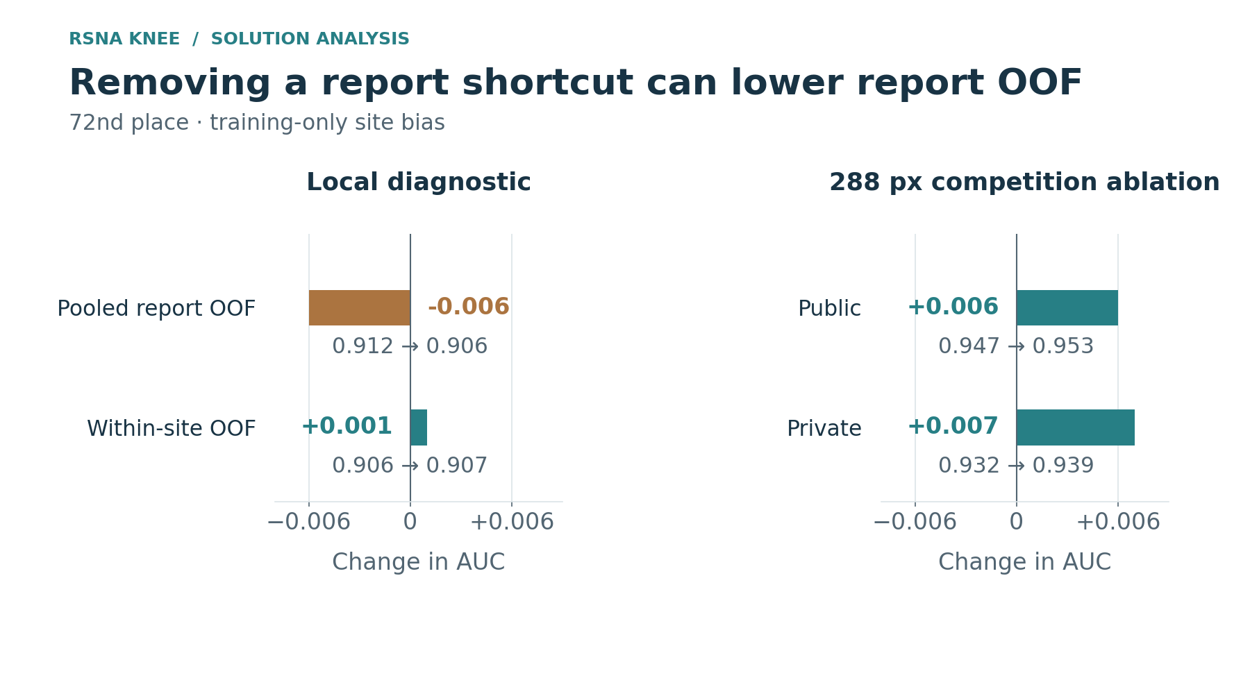
Figure 5. The 72nd-place report-reference diagnostics and its exact 288-pixel site-only competition comparison. Pooled/within-site local references differ from the expert competition annotations. Private was revealed after the deadline.

The later pseudo-label results also limit the within-site interpretation. The author’s within-site winner used a lineage with inflated OOF and reached only 0.942 Private, below the final model. Within-site scoring still needed compatible label ancestry; changing the aggregation did not repair leakage in the predictions being scored.

The 22nd-place author took a different route: five-fold predictions on 4,342 studies were scored against one fixed Astra image-reading reference. Training-label changes did not redefine the reference. The author wrote acceptance rules before experiments and recorded local and Public deltas whenever a differently supervised member entered. One main-label replacement gave +0.0031 locally and +0.003 Public.⁷ That agreement supported that comparison; it did not turn the VLM reference into an independent clinical answer key.

The first-place team’s late development system also fixed its image-assisted reference but used a different metric. Sakaku held out one 435-study fold, chosen from ten candidate folds for agreement with historical LB, and trained on the remaining 3,914 report studies plus 58 expert cases. Its probability-weighted SoftAUC was

\[\operatorname{SoftAUC}(p,q)= \frac{\sum_{i\ne j}q_i(1-q_j) \left[\mathbf1(p_i>p_j)+\tfrac12\mathbf1(p_i=p_j)\right]} {\sum_{i\ne j}q_i(1-q_j)}.\]

This preserves uncertain reference probabilities instead of thresholding them. Its scale differs from hard-label AUC. It was a single development fold selected using earlier leaderboard results, not ten-fold averaged CV and not an independent test. Tascj’s account likewise described comparing candidate reference scores with historical Public results.⁸¹⁴ The useful practice was fixing a reference for a decision; the selection history must remain attached to its claimed reliability.

Gold-58, selection uncertainty, and prior exposure

The 58 expert studies supplied direct information about the target definitions, but not enough independent examples to rank every nearby model. Authors reported only 9–35 positives per finding. For a target with nine positives, every positive affects many positive–negative pairs; one ambiguous case can change an apparent model preference. Macro averaging does not create more independent patients.

The 49th-place account estimated paired gold macro variation around 0.0125, and seed variation around 0.0026 in its fold experiments. The 74th-place account reported gold bootstrap SD around 0.016. These are different statistics and experimental settings, not interchangeable constants. Paired resampling is often more informative than comparing two independent confidence intervals because it retains shared difficult cases, but a narrow paired interval still conditions on the chosen cases and reference.¹⁶¹¹

The second-place team’s tune/check split exposed a specific failure. Additional blind single-finding reads improved the 24 tuning cases by 0.066 and worsened the 34 checking cases by 0.019. It also explicitly disclosed that later rules, including its PF OA floor, used all 58. A useful split earlier in development does not make every subsequent score on those same cases held out.³

The first-place reading-guide comparison provides another distinction. Fitting and applying a guide on the same 58 produced 0.943 AUC; its out-of-fold application reported 0.936. That fold exclusion addresses fitting the guide from the expert answers. It does not erase earlier prompt, rubric, image-selection, or annotation design feedback involving the same cases. Sakaku’s new account made the boundary explicit: its production annotation did not directly inject the answer key, while earlier development had used gold feedback.¹⁴⁸

The 74th-place solution changed the role of gold after early selection failed. Gold-based epoch and weight choices improved gold by approximately 0.003 but reduced LB by 0.001. It subsequently used paired checks, leave-one-out sensitivity, and random half-splits primarily to screen large regressions, while external panels helped choose members. Its two selected candidates reversed the gold preference: 0.947 gold / 0.948 Private versus 0.942 gold / 0.949 Private.¹¹

Gold remained useful for distinguishing different label interpretations, exposing confident mistakes, and checking whether an extractor answered the intended clinical question. After repeated development use, however, it offered much weaker support for choosing between blends separated by one-thousandth. That distinction concerns the role of the panel, not whether expert annotations are valuable.

External expert sets were also conditional evidence. The 246th-place author used 2,399 OAI knees and three OAI-free models to test OA decorrelation, with an opposite-sign control and a predeclared rule. The direction replicated, but raw OAI overstated transfer because its compartments were much less coupled than the competition’s expert cases. Reweighting for coupling changed the predicted magnitude substantially. The 21st-place author similarly separated OAI MOAKS, WORMS, and KneeMRI checks rather than treating them as another copy of the twelve competition labels.²⁸⁶

Training exclusion and selection exposure are separate properties. An external panel is independent of training only if the model and its ancestors excluded it; its feedback begins to influence selection as soon as it changes the next choice. Keeping these sources distinct preserves their diagnostic value without treating every local score as an interchangeable estimate of the same quantity.

Uncertainty belongs to a comparison, not a score

The various reported noise estimates describe different repetitions. A patient bootstrap asks what happens if the evaluation cases change while predictions remain fixed. A new training seed asks what happens if optimization and sampling change while the evaluation cases remain fixed. An independent label reader changes the target construction. None is a substitute for the other two.

Let $D$ be a candidate-minus-control score difference, $U$ training randomness, and $B$ evaluation-case sampling under a declared protocol. The law of total variance gives

\[\operatorname{Var}(D) =\mathbb E_U\!\left[\operatorname{Var}(D\mid U)\right] +\operatorname{Var}_U\!\left(\mathbb E[D\mid U]\right).\]

A bootstrap of one trained candidate and one control addresses the first term conditionally on those fitted models. It does not estimate how much their difference changes under a different training draw. Conversely, two seed repeats on one reused expert panel do not establish transfer to a new panel. The equation is useful because it names the omitted source of uncertainty; it does not justify adding unrelated published standard deviations in quadrature.

The unit of resampling matters as well. AUC averages positive–negative pairs, but its pair terms are not independent: one patient appears in many comparisons. With nine positives, a suspicious positive study influences its comparison with every negative. Treating the number of pairs as the number of independent clinical observations would make the apparent precision far too high. The 21st-place continuation comparison resampled patient/report groups, retaining the dependence that its split construction was meant to respect. Finding-level analyses need to retain relevant grouping and declare how undefined AUCs are handled when a resample loses one class.

A paired design removes some avoidable variation. If candidate and control use the same fold assignments, update budget, and inference coverage, their difference is easier to interpret than the difference between two unrelated best runs. It does not remove all uncertainty: changing labels changes the optimization trajectory, and different cases may benefit in opposite directions. Replication across another fold or seed can test whether the observed mechanism survives those changes without pretending that the repeats are new expert labels.

The 77th-place author’s approximately 0.0025 seed movement and its decision rule around 0.002 were local operational choices. The 22nd-place author reported approximately 0.003 seed variability, with substantially larger variation for lateral OA in compartment models. Their numbers have different models and targets behind them. I should not inherit the cutoff from the more successful team and call it a property of this competition’s AUC.¹²⁷

There is also bias that a variance estimate cannot repair. If both the candidate and its evaluator reproduce the same report convention, a very narrow confidence interval can establish the wrong improvement accurately. If 30 variants were explored and only the best interval is shown, the interval is conditional on a selected comparison. If an expert panel helped write the annotation protocol, splitting the panel afterwards does not undo that use. Each is a different reason a convincing-looking local result may fail to transfer.

Uncertainty therefore has to be assessed for the particular comparison. A small effect can remain useful when its mechanism and deployment cost are favorable; a larger local effect can be misleading when it comes from a reference shortcut or a broken decoder. The effect, relevant repetitions, and unresolved discrepancies belong together. One fixed minimum detectable difference cannot summarize them all.

Distillation targets and the complete exclusion boundary

Teacher predictions can contribute visual evidence, smooth an uncertain target, or simply reproduce the mistakes of their training labels. The names “OOF teacher” and “self-distillation” do not establish which of those happened. The evaluation boundary has to follow the complete estimator.

The 21st-place solution used a valid but easily misdescribed arrangement. For outer fold $k$, let $T_k$ be the training partition and $V_k$ the validation partition. A teacher trained on $T_k$ predicted those same training rows. The student target was

\[q_i^{(k)}=0.75q_i+0.25t_k(x_i),\qquad i\in T_k.\]

The student also trained only on $T_k$; both models excluded $V_k$. The teacher targets were in-sample inside the outer training partition, not inner OOF. They could still support an outer-held-out student comparison. Dense teacher inference and center crops supplied stable probabilities, whereas the student trained with sampled windows and augmentation. An inner OOF teacher was not a prerequisite for that specific question.⁶

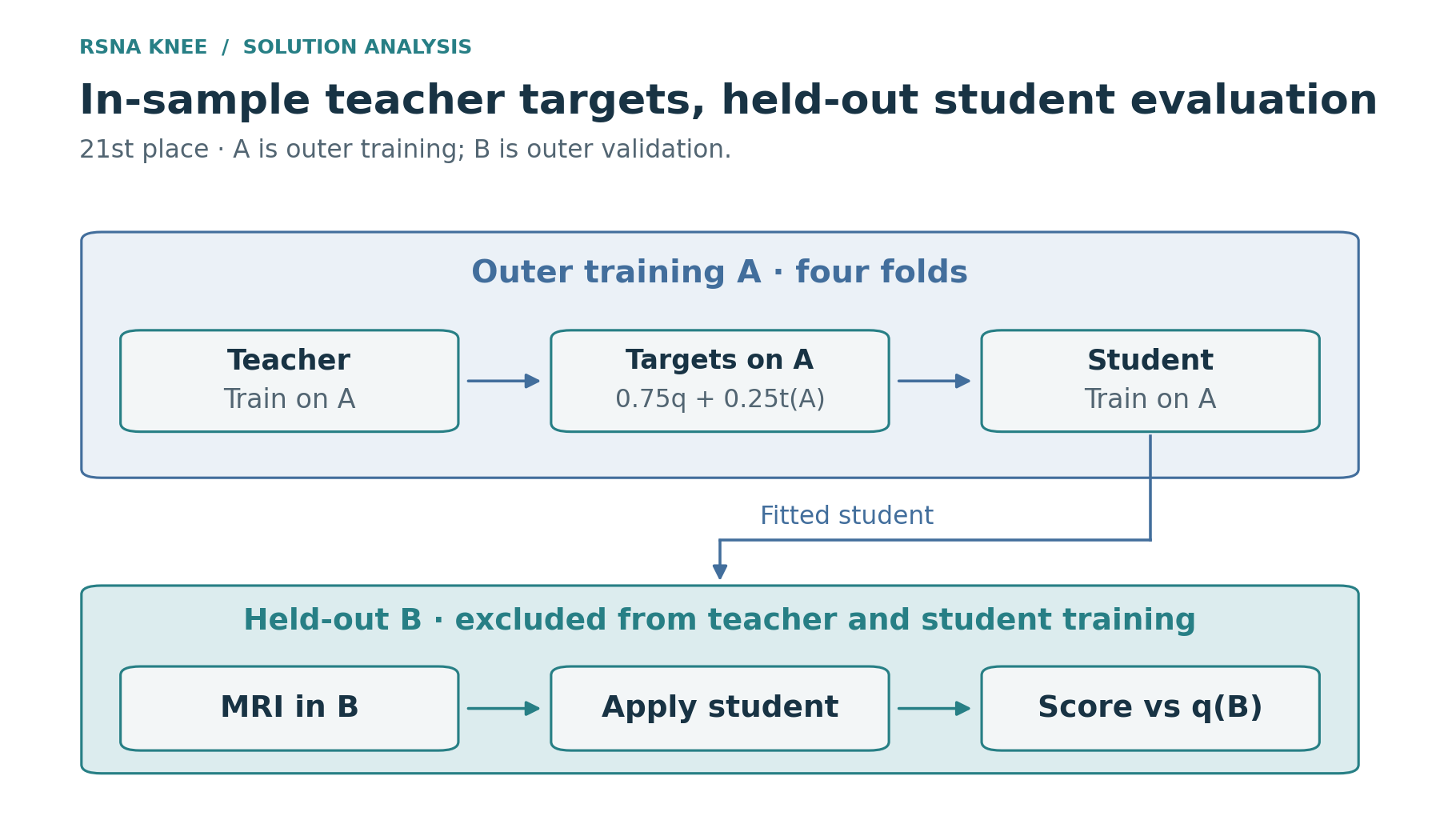
Figure 6. The 21st-place teacher predicts its own outer-training rows. Both teacher and student exclude the outer validation fold; evaluation uses the original LLM reference. Upstream annotation and selection exposure are separate boundaries.

The author matched continuation from the same checkpoint for two epochs: one arm retained LLM targets, the other used distillation targets. The reported extra OOF gain was 0.000477, with a patient/report-group bootstrap interval [0.000112, 0.000900]. The reported delta is retained here; subtracting the displayed endpoints gives 0.000478. Gold changed little. A completely retrained student then scored 0.958492 LLM-reference OOF / 0.940240 gold / 0.963 Public, compared with 0.960760 / 0.943083 / 0.962 for the LLM-only continuation. The better local continuation was not the better Public model.

The dangerous arrangement is different: a teacher used to construct targets for $T_k$ has itself learned from $V_k$, or its calibration and transformation were fitted using validation answers. The student can then inherit the held-out information without ever directly training on the original validation rows. A global OOF table may exclude each row from its own producer yet remain unsuitable for a later outer evaluation that requires a whole fold to be unseen throughout the pipeline.

The 49th-place account quantified this in a sealed-fold audit. Excluding fold 3 from every teacher yielded approximately +0.004 on report validation for one label round; the global-teacher construction showed about +0.011. The larger local gain was not three times the scientific progress. The 478th-place account likewise reported held-out report AUC rising 0.923 → 0.931 while LB stayed flat, with later teachers having trained on that fold.¹⁶²⁹

The same distinction applies to my teacher descendants. Clean folds in an image student do not remove information inherited from a full-data public parent in its targets. Those descendants can be useful final predictors, while their local scores remain ineligible as clean held-out estimates of the whole pipeline. Conversely, an outer-training-only teacher already supports the specific student comparison above; requiring nested teacher OOF for that question would add work without changing its exclusion boundary.

Repeated teacher rounds, calibration, and shared errors

The eighth-place team found that class weighting and ranking losses had moved teacher means to 0.37–0.46, while its label means ranged 0.10–0.40. Averaging those probabilities without checking scale would partly redefine the target through the teacher’s loss. It fitted per-finding isotonic regressions on the other three folds before correcting a fold’s predictions, then mixed calibrated OOF back into a fixed original source $S$:⁵

\[q^{(t+1)}=0.6S+0.4\widehat p^{(t)}_{\mathrm{OOF,cal}}.\]

Reusing the previous target instead would reduce the direct original coefficient to $0.6^2=0.36$ after a second round. Keeping $S$ fixed makes that change explicit. It does not remove errors indirectly transmitted through the teacher, and isotonic calibration itself has a training/validation ancestry. The fixed anchor is an accounting choice with a testable consequence, not a proof against drift.

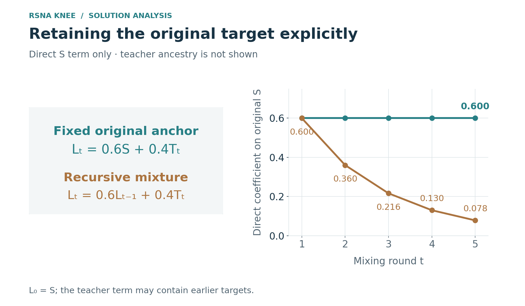
Figure 7. The explicit original-source coefficient outside the teacher is 0.6 each round with a fixed source, versus 0.6 raised to the round number when the previous target is mixed recursively. This is not the total ancestry influence: teachers can carry the original source indirectly.

The reported outcomes varied enough to reject a universal “one more teacher round” rule:

Solution	Useful reported change	Limitation or counterexample
49th	Five-fold teacher rounds improved matched Public comparisons	A larger teacher sharing the same text lineage gave a flat round
72nd	One teacher per report source improved Private 0.923 → 0.931	More text extractors and another strong-student round did not help
76th	Gold-fine-tuned teachers propagated the expert convention	A fourth generation and additional pseudo-labeled OAI images tied their controls
77th	OOF-mixed labels improved several student backbones	ConvNeXt-T showed no Public improvement from that relabeling
478th	First-round student ensemble improved Private 0.933 → 0.938	Later rounds, higher teacher shares, and about 10,000 fastMRI studies did not move the result

The 76th-place recipe illustrates why “new information” can have a precise meaning. Its teacher heads were first fine-tuned on the expert cases, then their predictions were spread to report-only studies. That changes the source of supervision, although it also spends the gold set and limits its later role as an independent evaluator. Its largest reported gain came early; a higher 75% teacher share was not better than 50%.³⁰

In the 74th-place account, several rounds and additional models plateaued because their targets were partly produced by the same earlier models. Independent OAI readers helped correct selected findings, but they over-coupled medial meniscus and medial OA and were rejected for those targets. Same-budget continuation controls attributed part of the improvement to the corrected labels rather than merely extra epochs.¹¹

Different encoders can learn complementary approximations of one teacher, but those approximations are not independent diagnostic evidence. The reported plateaus distinguish two possible benefits of another round: fitting the existing signal more effectively, or incorporating a genuinely changed source. Same-budget continuation controls and parent-specific error comparisons help separate them.

Public comparisons, target probes, and repeated selection

The overall Public–Private ordering was strong, but aggregate agreement was not a calibration of every small candidate difference. The second-place team reported rank correlation 0.977 among its later submissions; the 72nd-place author reported 0.94 across 26 single models. A set spanning weak and strong systems can have excellent correlation while still reversing two nearby ensembles. It also cannot establish a universal 0.003 boundary below which information vanishes or above which a comparison is reliable.³¹⁸

Public could answer narrower questions when the submission operator was declared in advance. If the other eleven columns are constant 0.5, a single-finding probe has

\[M_{\mathrm{probe}}=\frac{A_c+11/2}{12}, \qquad A_c=12M_{\mathrm{probe}}-5.5.\]

The eighth-place team used this identity. A displayed macro step of 0.001 becomes a 0.012 step in the inferred target AUC. The 49th-place approach instead inverted one column of a fixed base prediction. Because inversion changes $A_c$ to $1-A_c$, including half-credit ties,

\[A_c=\tfrac12+6(M_{\mathrm{base}}-M_{\mathrm{inverted}}).\]

If each macro score is rounded to the nearest 0.001, the constant-column probe has a worst-case rounding error of 0.006 after multiplication by twelve. The inverted-column estimate has the same 0.006 bound: two rounding errors can differ by 0.001, then the factor of six applies. This is a bound on display rounding alone, not a confidence interval for sampling or training variation.

These are algebraic consequences of macro AUC, not ways to recover unlimited test precision. Display rounding is magnified, and every probe uses the same Public cases. The method is better suited to locating a weak finding or testing a predeclared specialist than searching many target weights.⁵¹⁶

The second-place specialists show both outcomes. Its PF OA specialist improved the target probe from 0.920 to 0.944 Public and approximately 0.908 to 0.932 Private against the stated comparator. Its lateral specialist improved Public 0.920 → 0.932, yet later scored roughly 0.944 Private versus 0.956 for the core member. A useful probe can still select the wrong close alternative on unseen cases.³

The 228th-place sequence makes the repeated-selection cost visible. Its first mechanism-backed debiasing candidate scored 0.960/0.945; roughly 25 similar refinements produced a selected 0.961/0.944. The basic correction transferred, but the Public-best refinement did not. The 63rd-place author likewise reported tuned per-finding weights at 0.958/0.942, compared with 0.960/0.948 for its uniform-weight alternative.²⁷²⁴

Public was useful when a declared comparison tested transfer, a specialist, or a reporting correction. Neither broad rank correlation nor a finely optimized sequence of rounded scores could settle every nearby choice. Adding a successful predictor to an existing parent poses a further question: whether their joint predictions repair errors that the parent still makes.

4. Prediction banks and final composition

Standalone strength and marginal information

A useful family has two separate properties: how well it predicts by itself and which errors it can correct in another predictor. Strong standalone performance makes it a promising basis. Complementary ordering errors determine whether it is a useful addition. Architecture names, parameter counts, and the number of completed runs are indirect descriptions of those properties.

For one binary finding, let a base predictor assign scores $b_i$ and a candidate assign $u_i$. In a simple score mixture with weight $w$, the margin of a positive case $i$ over a negative case $j$ is

\[m_{ij}(w)=(1-w)(b_i-b_j)+w(u_i-u_j).\]

The corresponding change in AUC is

\[\Delta\mathrm{AUC}(w) =\frac{1}{n_+n_-}\sum_{i:Y_i=1}\sum_{j:Y_j=0} \left[H\!\left(m_{ij}(w)\right)-H\!\left(m_{ij}(0)\right)\right],\]

where $H(a)$ is 1 when $a>0$, 0 when $a<0$, and 0.5 at a tie. A candidate helps when its added ordering corrects enough pairs without overturning too many correct ones. High correlation with the base does not prove zero value: a small set of repaired pairs can matter. Low correlation does not prove value either: many of the changed pairs may become worse.

This is why general diversity statistics are useful diagnostics rather than an ensemble objective. A model can be different because it sees another view of the knee, because it has a better target, because it is poorly calibrated, or because it is simply noisy. Pairwise error behavior on a compatible reference helps separate those explanations. It remains conditional on that reference: diversity measured against report labels is not automatically diversity against the expert target.

Even equal standalone AUC does not fix the result of averaging. Consider a four-study binary example with the first two entries positive and the last two negative. Base scores $(0.9,0.4,0.6,0.1)$ have AUC 0.75. Candidate scores $(0.5,0.9,0.1,0.6)$ also have AUC 0.75, but the equal score average ranks both positives above both negatives and reaches AUC 1.0. In a second example, two score vectors $(0.9,0.4,0.8,0.1)$ and $(0.4,0.9,0.8,0.1)$ each again score 0.75; their probability average puts the shared hard negative above both positives and scores 0.5. The component AUCs alone do not reveal the decisive margin structure.

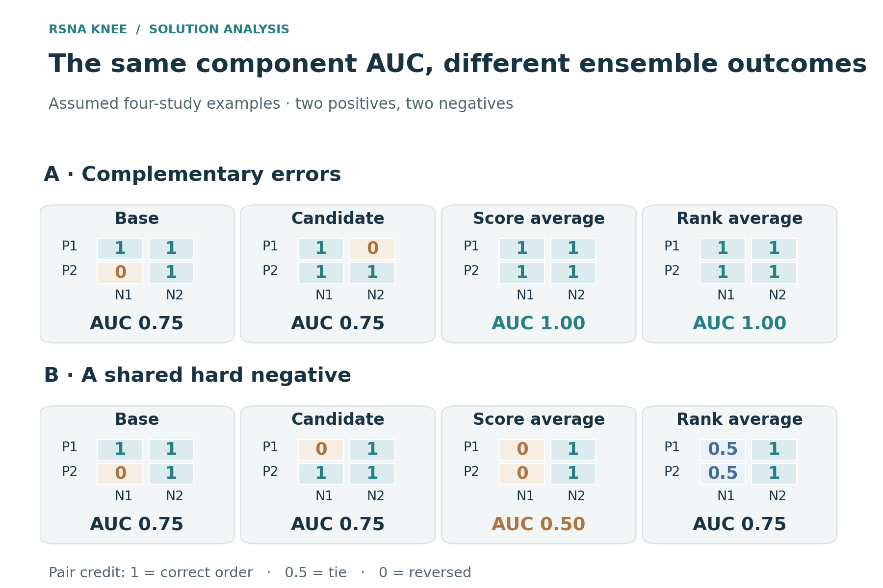
Figure 8. Toy binary examples, with the first two studies positive and the last two negative. Both components have AUC 0.75 in each example. Their raw score average can reach 1.0 or fall to 0.5; changing the operator can change that result.

My complete OOF bank made these comparisons possible without another full training campaign: margins, folds, targets, and alternative compositions were already available. Its size did not ensure that it contained a sufficiently strong or complementary source. Students of a common teacher could add many prediction files while retaining much the same hard-negative structure.

Probability, logit, and rank mixtures

Three common operators average different quantities. For model probabilities $p_{m,c}(x)$ and nonnegative weights summing to one,

\[p_c^{\mathrm{prob}}(x)=\sum_m w_{m,c}p_{m,c}(x),\]

whereas logit averaging gives

\[p_c^{\mathrm{logit}}(x) =\sigma\!\left(\sum_m w_{m,c}\operatorname{logit}p_{m,c}(x)\right).\]

Logit averaging requires probabilities strictly between zero and one, or a declared clipping rule for the endpoints. Numerical clipping is part of that operator, not a new calibration result.

A rank mixture first replaces each score with its position in an evaluation batch $B$:

\[\rho_B(p_i)=\frac{\operatorname{rank}_{B,\mathrm{average}}(p_i)}{|B|}, \qquad s_{i,c}^{\mathrm{rank}}=\sum_m w_{m,c}\rho_B(p_{m,i,c}).\]

A strictly increasing transform preserves an individual predictor’s AUC, but mixing transformed scores need not preserve the mixture’s ranking. In a probability average, a model with a wide probability range has more numerical influence than one with compressed outputs. Rank conversion removes much of that scale difference while discarding score spacing; logit averaging emphasizes confidence differently. The choice of AUC as the final metric does not make those operators equivalent.

This was visible in the published systems. The 21st-place final averaged fold logits within each own family, applied sigmoid, and then mixed family probabilities with fixed weights of 0.45, 0.45, and 0.10 for the public contribution. The 302nd-place account used standardized logits rather than percentile ranks when adding its own models to a public base. Many public-stack extensions instead used multiple stages of ranks. These are distinct estimators, even if their ingredient lists name the same architecture families.⁶³¹

Rank mixtures have an additional implementation property: they depend on the batch of studies being ranked. A rank-based whole-cohort predictor cannot always be replayed by independently processing a few cases and assuming that the final mixed values are comparable. Relative ranks within each component change with the cohort, and the mixture uses those relative locations. The 499th-place team ran 104 training studies—the 58 expert studies plus 46 other studies—to exercise a production rank branch intended for more than 100 rows. That made its replay more faithful to the implementation, while the 58 expert cases still remained a repeatedly used development panel.³²

The practical consequence is that a saved CSV must be identified by more than its model names. Is it a raw probability, an average logit followed by sigmoid, a percentile, or an already ranked blend? Averaging a rank as though it were a calibrated probability changes both training and combination. A whole-bank search can optimize the wrong object very effectively if that distinction is lost.

A new arm changes both content and allocation

The public H family was a hierarchy, not one flat average. In a reduced version of its structure, the Raptor arm combines a 384-pixel predictor and a 224-pixel predictor at 0.65 and 0.35. A finding-specific weight then combines that arm with R6. The published 412th-place account gives Raptor shares of 0.8 for Synovitis, 0.6 for PF OA, 0.35 for Baker’s cyst, 0.2 for Lateral OA, and 0.5 elsewhere. A small reader injection forms another stage.³³

That structure makes the location of an added S6 predictor important. Suppose a simplified base, before its outer re-ranking and excluding the small reader, is

\[H_c=w_c A_c+(1-w_c)B_c,\]

with $A_c$ the Raptor-arm score and $B_c$ the R6-arm score. Replacing part of the R6 arm gives

\[H_c^{\mathrm{inside}} =w_c A_c+(1-w_c)\left[(1-\beta)B_c+\beta S_c\right].\]

The direct S6 coefficient at this stage is $(1-w_c)\beta$. If $\beta=0.3$, it is 0.06 for Synovitis, 0.12 for PF OA, 0.195 for Baker’s cyst, 0.24 for Lateral OA, and 0.15 for the other findings. Adding an S6 arm after the entire base instead uses a form such as

\[H_c^{\mathrm{outside}} =(1-\delta)\rho_B(H_c)+\delta\rho_B(S_c).\]

The latter changes the allocation of all existing arms and gives S6 the declared outer coefficient $\delta$ at that stage. With intervening rank transforms, those coefficients are not a complete measure of final influence. They are nevertheless enough to show that the two constructions ask different questions.

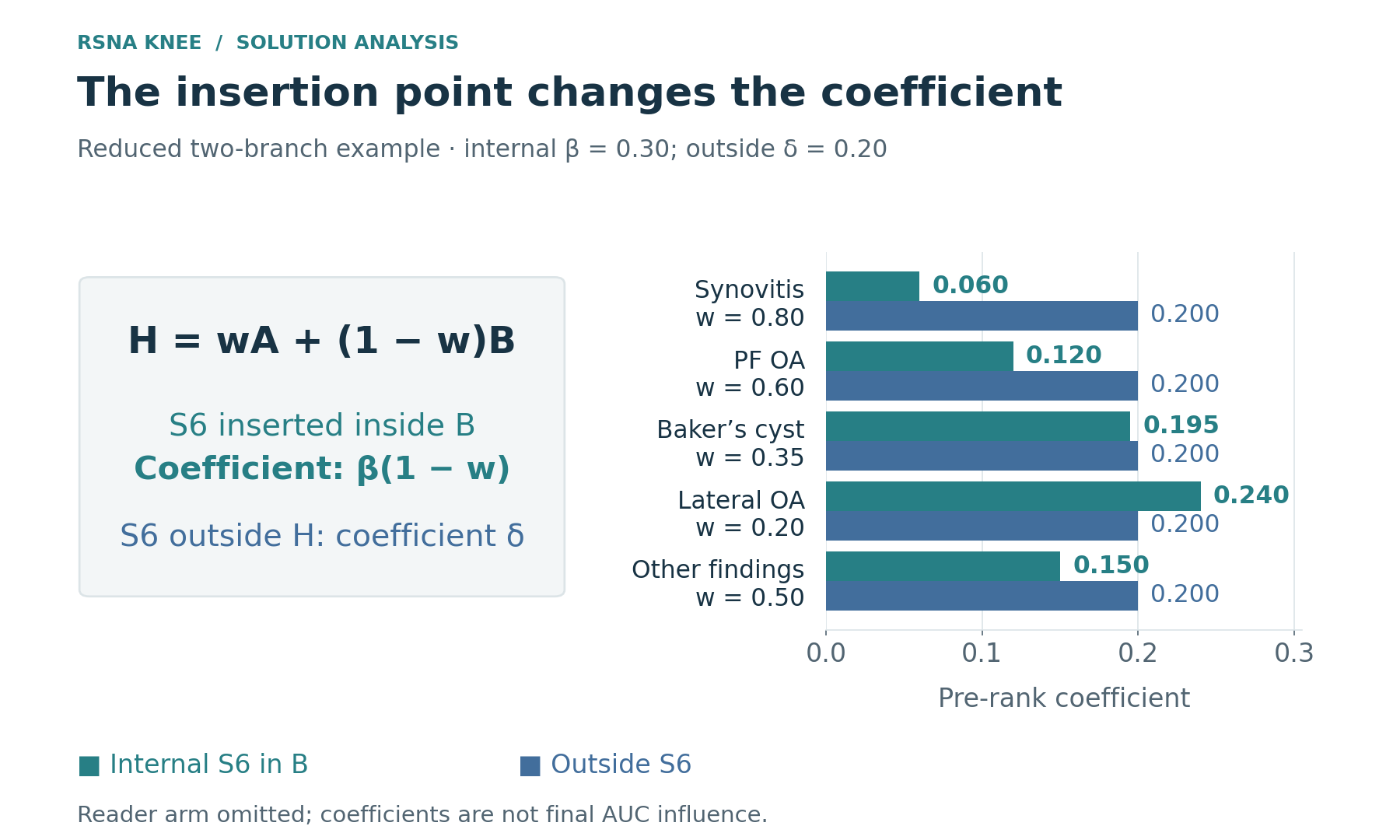
Figure 9. Direct coefficients in a reduced two-arm operator before outer re-ranking. An S6 weight of 0.3 inside R6 becomes 0.3 times the R6 share; an appended weight of 0.2 is a different allocation. The small reader is omitted from this algebraic comparison.

The Northstar team placed S6 inside the R6 half and finished with a displayed Private 0.942. The 412th-place team added S6 as an outer rank arm at 0.20 or 0.35 and obtained 0.943. The latter also retained a small reader that Northstar had tested only at much larger weights. This cross-team comparison therefore does not isolate placement as the cause of the score difference. Within the 412th-place author’s own controls, the public recipe went from 0.942 to 0.943 with the appended S6 arm. That is the relevant local evidence for the extension.³⁴³³

Adding a seed or family in my own packages could likewise change the total S6 share, the N/V3 balance, and outer rank normalization at once. The comparison measured that package change. It could support a useful coarse allocation decision without identifying an independent causal gain from the new checkpoint.

What the public-stack extensions actually contributed

Several middle-ranked solutions provide informative comparisons because they start from recognizable public parents. They show both the usefulness and the limits of adding another independently trained predictor.

Account	Own contribution or new arm	Matched Private observation
478th	Five-fold ConvNeXt-S student at outer weight 0.15	Public parent 0.942 → selected mixture 0.943
412th	Public S6 predictor appended at 0.20 or 0.35	Reproduced parent 0.942 → both selected mixtures 0.943
507th	Finding-specific base changes plus a retrained reader	Deployed parent 0.942 → selected variant 0.943
My submission	Own N/V3 rank block at outer weight 0.25	H parent 0.942 → selected mixture 0.943

The 478th-place student was reasonably strong by itself: Public 0.952 and Private 0.939. At 0.05 in the public mixture the displayed Private score remained 0.942; at 0.15 it reached 0.943. Later students, larger shares, and fastMRI-trained variants did not produce a higher displayed result. Replacing a fraction of R6 rather than appending the student was less successful. The author’s interpretation that public tuning partly concealed a Private contribution is plausible, but the paired results establish the narrower fact: this own model added a small amount to this parent under this operator.²⁹

The 507th-place team changed inherited finding weights and added a retrained 256-pixel reader. Its full-chain gold replay improved from 0.9384 to 0.9419 while Public declined from 0.958 to 0.957; Private moved from 0.942 to 0.943. The author treated the small gold advantage as a direction for selection, not an untouched verification. Both the reader and allocation changed, so the result cannot be attributed to either alone.³⁵

Larger own contributions sometimes achieved more. The 129th-place system used a 50% own rank block, with compartment-routed ConvNeXt, slice-context models, and a CoAt family, and finished at 0.946. The 243rd-place system reached a reported standalone Public 0.954 and placed its own model into half of the 2D allocation while preserving the public 3D R6 component; its final Private was 0.944. That description is more precise than calling the whole system an unconditional 50/50 blend. The 302nd-place account added eighteen own models, ten trained using expert-graded OAI knees, but its brief text does not give enough ablations to assign separate gains to the external data, model count, and standardized-logit operator.¹³³⁶³¹

The useful own share depended on the parent and operator. A 15% arm could help, a 50% arm could be justified, and a larger bank could add nothing. Those weights describe hypotheses about complementary errors, not independent evidence or an entitlement to final membership.

A different route appears in the 215th-place account. Its own RadImageNet-based arm contributed 25% of a public mixture, followed by partial rank correction within magnetic-field-strength groups. Moving from no final field correction to a 0.35 correction changed Public from 0.958 to 0.960; increasing that correction to 0.5 reduced it to 0.957. The selected full system scored Private 0.944, but the account does not supply a matched Private delta for the field correction itself.³⁷

That operation is also transductive: each test group’s score distribution participates in the mapping. The author compared a train-fitted inductive version locally, but submitted the transductive route. Both versions differ from removing a training-only site logit. A distributional postprocessor can be a useful candidate when a concrete acquisition effect is suspected; it is not an automatically valid normalization of every test group. Genuine prevalence and severity differences can be part of the signal, and a missing DICOM tag needs its own treatment rather than an invented field strength.

Adaptation can occur in weight space

The 220th-place team took another route. Rather than only adding a new prediction file, it fine-tuned public checkpoints for one epoch, explicitly sampled the 58 expert studies into batches, and averaged resulting parameters with the originals. Its reported soup for the main reader was

\[\theta_{\mathrm{soup}} =0.25\theta_0+\sum_{r=1}^{4}0.1875\theta_r.\]

The coefficients sum to one, but a parameter average is not the same operation as averaging the five prediction functions. The fine-tunes share an architecture and a nearby initialization; that makes local parameter averaging meaningful in a way that averaging unrelated model families would not be. The submitted system also included other readers, specialists, and a 3D contribution. Its 0.944 Private result is a package result, not a measurement of the soup alone.³⁸

This matters when interpreting the negative fine-tuning result from Northstar. The team reproduced the original nartaa inference at Private 0.930, then fine-tuned on its own labels and an 80% training split, obtaining 0.926. The result is evidence that that adaptation weakened the predictor. It does not prove that every adaptation of the public checkpoint is harmful. The label target, available data, gold exposure, schedule, and parameter averaging all differ from the 220th-place route.³⁴

Public weights offered several distinct paths: a final-only anchor, a clean reproduction of the code, revised supervision, controlled fine-tuning, or a teacher. Each produced a different asset and required a different evaluation boundary; “public” versus “own” was too coarse a distinction to choose between them.

Single-model strength and ensemble size

Published results do not support a rule that a compact ensemble always wins. The first-place final combined seventeen classification checkpoints in one branch with three full-data models in another. The 22nd-place solution used 56 networks across several groups. Those are substantial ensembles. Their strong individual routes and complementary target-specific views made the size useful.

Other results show saturation. The seventh-place author reported one full-data ConvNeXt-S model at Private 0.958 versus the final ensemble at 0.957. The 72nd-place final was itself a five-fold family; blends with older models were worse. The fifth-place best M3 family matched the displayed final score at 0.958. The latter two examples compare fold ensembles with larger compositions: a five-fold family already averages several checkpoints.

My bank needed to support both additions and replacements, including removal of a weak component, while preserving unselected complete clean families. Restricting search to the recorded package plus one member would make earlier choices define the entire search space. A broader search could improve selection within the bank; it could not create the stronger features or supervision that the bank still lacked. That was the distinction between improving the composition and changing the next research investment.

5. Research decisions I should have changed

The technical differences above changed what was worth investigating next. Better targets could strengthen an existing inference route; a wider view could expose evidence that another backbone could not recover; a reporting shortcut could make a higher local score actively misleading. I had enough of these signals to question the research programme before the final results. Too often, I kept improving the established pipeline rather than testing the uncertainty that limited it.

The recurring error was a mismatch between the scope of an observation and the decision it supported. A clean prediction was not necessarily scored against the right target. A negative pilot was not a verdict on every implementation of its idea. A larger bank was not proof of more independent information. Correcting those inferences would have changed both the next comparison and the work it displaced.

Target definition and label construction

The report-label discrepancies identify three different questions: did the extractor reproduce the report, did the report contain the finding, and did its description meet the competition criterion? I should have diagnosed which question had failed before buying another annotation pass. Incorrect extraction called for an extractor repair; an omitted finding required another information source; a severity mismatch required a target-definition correction. If the student could not see a small lesion, the input also had to change. Another pass over the same report could not solve all four.¹³

The useful comparison was a fixed student trained on two target constructions. One retained the report-derived targets. The other corrected a defined failure, such as low-grade abnormalities treated as positives or image-visible findings absent from the text. Student, folds, update budget, and inference coverage would remain fixed. Disagreement cases could reveal what the correction changed; a random sample could show how often the problem occurred. Handpicked disagreements alone would not establish its population value.

Controls then needed to distinguish the remaining explanations. Swapping images tests whether the reader responds to visual input; reviewing a cited slice tests whether the answer refers to the relevant anatomy. Neither establishes downstream prediction value. A matched student was still needed before a promising annotation became a reason to relabel the corpus.

A larger campaign would be justified if that student benefited and the remaining errors pointed to information the revised reader could recover. Repeated old answers, evidence unavailable to the student, or a gain that disappeared under an applicable evaluation would instead call for redesign or a different information source. The same distinction applies to a churn target affected by follow-up duration or a text target based on moderator action: fitting the recorded outcome can be useful, but does not by itself validate a claim about another outcome.

Ranking quality and training probabilities

The probability analyses reveal a second mistake in how I assessed labels. AUC is unchanged under a strictly increasing transform of a model’s output, but a transformed soft BCE target gives the student different instructions. The derivative $p-q$ makes the distinction explicit: changing the confidence of $q$ changes the gradient even when its ordering across studies is unchanged.

A good label-table AUC therefore could not replace an investigation of probability quality. Confident wrong positives, values near one-half, and missing annotations affect learning differently. The stronger experiment would keep the image learner fixed while changing a justified mapping—for example, preserving explicit negatives, masking actual missing responses, or reducing confidence in a report group known to disagree with expert criteria. I needed to inspect the frequency of each state and the cases whose gradients would change most.

Expert-fitted calibration would require the relevant fold exclusions, with any earlier use of those cases in recipe design recorded as development exposure. The first- and fifth-place analyses show how to investigate the problem, not a transform I could safely copy into my own labels.¹⁴¹ A matched student would decide its value. The general rule is to evaluate a representation by the operation that consumes it: a distillation target, propensity weight, ordinal regression outcome, and rank blend do not require identical properties merely because they are all numbers.

Pilot scope and follow-up experiments

H1c was already a controlled image-assisted experiment. It included report-only comparisons, repeated reads, and substituted images, followed by matched five-fold students; mm12 reached Public 0.914 against the control’s 0.911. The unresolved question was why the benefit was limited. Some outputs responded to the correct and wrong images, while contusion remained strongly report-dependent. That pattern warranted investigation of coverage and grounding, rather than a broad conclusion about the ceiling of image-assisted supervision.

The next comparison should have varied the view while retaining the diagnostic definition: a fixed packet against broader series coverage or targeted reinspection. Keeping the reader fixed first would isolate coverage; a stronger complete reader recipe remained a reasonable alternative if that comparison could not resolve the limitation. A small challenge set of localized marrow findings could test whether the interface exposed the required evidence, while a separate random sample could indicate its wider importance. Only then would a matched student show whether the improved annotation was useful for learning.

Solving handpicked failures alone would not justify annotating the whole corpus. Credible performance on both samples, followed by useful student transfer, would justify expansion. Adequate coverage and a compatible student that still failed would support stopping the route or changing its information source.

This gives a pilot a stopping rule without turning every early failure into a method-wide rejection. Irrecoverable geometry, unusable images, a learner unable to consume the signal, or an unaffordable delivery chain can end a route. A short checkpoint below the incumbent is weaker evidence against a different learning system unless their early-to-final behavior is known to be comparable. Rejecting retrieval after testing a weak retriever with truncated documents would make the same inferential mistake: the configuration failed, but the broader claim was not yet tested.

Coherent recipes and component tests

Early architecture changes were tested inside a DINOv2-oriented recipe, and poor drop-in results weighed against much broader alternatives. The September learning-rate × fine-tuning-depth diagnostic showed that changes could interact strongly even within one architecture. It did not prove another backbone would succeed. It showed why isolated substitutions were insufficient to characterize a coupled recipe.

A serious alternative first needed a coherent implementation with its intended supervision, physical coverage, normalization, aggregation, and optimization. Its inputs and prediction path had to be checked well enough to distinguish a failed reproduction from a properly implemented method that did not transfer. If the complete comparison was promising, removing or replacing costly components could identify what deserved further investment. Repeated infrastructure failures would not count as independent scientific negatives.

The reader-and-coverage question illustrates the sequence. Let $a$ select the old or revised reader and $b$ the compact or broader annotation packet. Each cell trains the same student recipe and is evaluated against the same eligible reference, giving score $S_{ab}$. The interaction contrast is

\[I=(S_{11}-S_{10})-(S_{01}-S_{00}).\]

It asks whether coverage has the same effect under both readers. Labels must be regenerated for the relevant cell; student splits, update budget, inference settings, and scoring stay fixed. Annotation cost belongs beside each cell. Repeated fits can test whether the interaction persists, whereas four displayed scores alone provide no uncertainty estimate.

All four cells need not be purchased before trying a credible system. The first comparison could be the coherent diagonal, $S_{11}$ against $S_{00}$. A gain would initially support the combined recipe and justify checking whether its expensive coverage expansion was necessary. A failure would require distinguishing inadequate information use from a valid negative; additional controls would separate the ingredients when that answer changed the next investment.

The second-place result is evidence for a better reader-plus-coverage recipe, not the causal effect of adding slices alone.³ My next comparison needed the same distinction. A strong end-to-end system could justify one serious reproduction without every component first winning as an incompatible drop-in, subject to full cost, readiness, and the alternative displaced. Tokenization and pretraining, missing-value semantics and feature construction, or a retriever and context window can interact in the same way. Factorial precision is useful when it resolves a decision; it is premature when neither baseline faithfully represents the system being judged.

OOF-bank breadth and information diversity

In the early bank, 57 of 66 completed OOF runs were DINOv2-small label variants sharing the same basic input. An August diagnostic had already found that the ensemble gain available in that bank was much smaller than the gap I was trying to close. This was a warning about saturation in the examined bank, not a ceiling on ensembles. Yet expanding its entries remained easier than building a stronger source of prediction information.

For K equally weighted predictors, write member $m$’s probability error as a shared component plus a member-specific component:

\[e_m(x)=b(x)+u_m(x),\qquad \bar e(x)=b(x)+\frac{1}{K}\sum_{m=1}^{K}u_m(x).\]

Averaging changes the second term while retaining the common component in this decomposition. The true components were not observed, and this is not an AUC forecast. It expresses the limitation suggested by the pair-order examples: numerical disagreement can coexist with the same omitted findings or hard-negative errors. Seeds, nearby label mixtures, and students of one teacher may improve approximation without supplying another information channel.

The next investment therefore needed two comparisons: against the strongest standalone family, and against the actual deployable parent. A better target, a view exposing missed anatomy, or a coherent stronger learner could raise the first frontier, improve complementary errors, reduce cost, or enable a replacement. Low global correlation alone established none of these. A strong standalone model and a weaker complementary model could both remain useful in whole-bank searches.

Preserving complete families did not require indefinitely expanding their lineages. Repeated matched saturation plus a ready alternative should have redirected new work. Finishing a nearly complete useful family could still be sensible without filling the next week with descendants. In time series, many window variants can share a regime failure; sampling the same history again differs from adding a genuinely new predictor available at prediction time. In tabular modeling, algorithms sharing an unavailable-at-inference feature do not provide independent confirmations. The diversity that matters lies in usable information and relevant errors.

Validation references and decision scope

My primary score looked useful across fourteen individual families on September 30. Across ten packages on October 6, its Pearson correlation with Public was −0.322. That small historical sample did not make Public infallible or invalidate OOF. It showed that success in one comparison class had not validated the reader as a selector for another.

The 72nd-place site intervention later provided a clear mechanism for such a reversal.¹⁸ A fixed report reference can compare optimizer changes within a label lineage while penalizing a correction of reporting habits. Its post-competition Private correlation analysis was unavailable during my development, but my own local/Public disagreement was already sufficient reason to investigate the reference and suspend its automatic package veto.

The reader scores should have remained conditional diagnostics. Their use needed a defined scope: source, excluded groups, label ancestry, prior exposure, and applicable comparisons. A label change should not be decided solely by agreement with the same label source; a near-identical seed comparison need not wait for an entirely new annotation system; a convenient local proxy does not turn a final-only public anchor into clean OOF.

Disagreement called for specific controls. Did the change improve within-site ordering but lose cross-site offsets? Did a decoder redefine positives? Did local inference use another crop or reducer? Did the candidate share the evaluator’s parent? Another aggregate correlation could not distinguish these possibilities. A compatible matched comparison could restore confidence for that decision class; choosing a new panel because it produced a preferred order could not. Evaluator work had to stop once it adequately supported the decision—or once its unresolved limitation was explicitly accepted—rather than freeze every bounded transfer test.

The transferable distinction is between the intended decision and the validation design. A random split may compare algorithms while missing a future regime; a familiar test suite may miss a changed interface. Neither problem is repaired by abandoning validation or granting another convenient metric universal authority.

Inconclusive results and default allocation

The September label comparison displayed Public 0.913 versus 0.911. The decision record acknowledged that it did not settle the predeclared boundary, yet the subsequent queue stayed on the existing labels. “Not enough evidence to switch” became an argument for continuing the default campaign.

The error was not that 0.002 had to be meaningful or meaningless. An uncertain contrast had settled a larger allocation without a separate justification. Nor did the expert-label preference justify switching every strong learner: the panel was small, exposed, and evaluated a different object. The comparison needed an unresolved branch.

That branch could have funded a stronger matched student on the competing targets, investigated the cases where target definitions disagreed, or tested useful teacher content against ordinary smoothing. Each option had to identify the work it delayed. Repeating a weak learner could remain uninformative if its input or capacity prevented it from exploiting the changed targets.

A predeclared rule needs actions for expansion, stopping or redesign, and unresolved evidence. The last can mean another discriminating comparison, a temporary default with an expiry condition, or no further work because the opportunity cost is too high. Retaining the incumbent may be sensible when transition costs are high or time is short. It is then a risk and scheduling choice, not a statistical finding of equivalence. Thresholds can limit reactive tuning without awarding the incumbent an unlimited budget; the remaining plausible benefit, evidence required, and competing project still matter.

Expert feedback and selection exposure

The expert-panel analyses above exposed a budget that GPU accounting missed: independent feedback. A case that revised the rubric, reader, calibration, epoch, and blend had influenced selection repeatedly even if its answer never entered a training loader.

I should have assigned the panel’s role before close comparisons. Some cases could support semantic diagnosis and target construction; an untouched subset could supply a limited check at its first inspection. If the panel was too small to split usefully, deliberate development use plus corroboration elsewhere could be preferable. Random half-splits after the same cases shaped the protocol would not reverse that exposure.

Expert calibration could improve the predictor enough to justify spending the panel. The error was claiming both that development benefit and an untouched test from the same feedback. Paired bootstrap measures sampling sensitivity conditional on fitted candidates; it does not replenish cases or test a changed annotation process.

A manually reviewed error set, a public benchmark used throughout prompt development, or a repeatedly inspected validation month poses the same problem. I need to track feedback that changed decisions, not just rows visible to gradient descent. When a close preference depends on heavily reused material, a simpler choice or another comparison is more useful than another decimal place on the same score.

Teacher transfer and ensemble contribution

My T* targets improved several standalone engines, while some corresponding parent-package comparisons improved much less or tied on the displayed Public score. That was evidence for better students, not additive ensemble gains or independently confirmed supervision. Regularization and improved fitting can help several architectures inherit the same useful knowledge and the same target errors.

The next generation required a fixed student architecture, schedule, and outer exclusions. Its original targets could be compared with one teacher mixture retaining an explicit fixed contribution from the original source, rather than recursively replacing that source with the previous mixture. A smoothing control would be appropriate if the question was whether teacher content added more than smoothing. In-sample inner-training teacher targets should be identified as such, while the complete estimator excludes the outer validation. A full-data public teacher that saw the outer cases, or unknown ancestry preventing exclusion, leaves final-only descendants.

Another generation would deserve funding if it changed errors relevant to the parent. Better fit to a teacher-derived reference, loss of a useful original signal, or no additional complementarity would instead call for a changed mixture or a different source. A new architecture name cannot erase that ancestry; repeatedly rephrasing one language teacher’s answers likewise does not create independent supervision.

Independence is not the only useful role. A student may replace a slower teacher, compress several members, or provide a cheaper approximation within the runtime limit. That requires speed-and-transfer evidence. It should not be sold as diversity, and a plateau should not automatically trigger more teacher rounds.

Public baselines and transfer comparisons

My hope that H’s advantage would disappear on Private was not borne out: it remained stronger than my completed own combination. This does not establish zero Public-selection optimism. During development, when Private was unavailable, the defensible response to an available predictor already ahead on Public was a small number of declared comparisons with a scored fallback—not discounting it on hope alone.

Provenance should have determined its role. A final-only release could be a deployable anchor, a starting point for clean reproduction, or evidence for a mechanism. Each required different work and allowed different claims. S6F later becoming my strongest complete family illustrated the value of reproducing a coherent recipe; it did not mean that exact training route had been ready weeks earlier.

Several of my Public comparisons already used a fixed coarse grid and a scored fallback. That discipline was worth retaining. For an own block added to H, the parent, membership, reducer, and allocation had to stay explicit: replacing an inner arm and appending an outer rank block tested different changes. A comparison of a fixed parent with one coherent arm could assess transfer or complementarity. Repeated tiny weights chosen after each result would increasingly adapt the decision to the same hidden subset. A favorable result supported the declared comparison, not every variant of the same method.

The next action should be written before submission for both outcomes. If the arm failed, I could keep H and stop that comparison without discarding clean OOF assets. If it helped, another small weight change still needed a reason to alter the final choice. When either outcome would lead to the same action, a selection test had little immediate value; a genuinely new source or mechanism could reopen the question later.

A comparator is a reference, not mandatory membership. Keeping a scored fallback while considering a replacement composition preserves earlier work without requiring the final predictor to justify the effort already spent on it.

Inference capacity and delivery cost

A research option needed a complete price. Annotation includes rendering, access, calls, recovery, quality checks, matched students, and integration. A new family needs sufficient training, complete folds where required, artifact recovery, and final materialization. An inference route includes decoding, transfers, compilation, memory behavior, aggregation, and valid output. Comparing isolated short jobs understated the work needed to obtain a selectable predictor.

Cost disclosures also need compatible boundaries. The second-place team’s approximately 100 GPU-hours covered final seed training, excluding research. My approximately 1,445 rented box-hours covered a much wider campaign. Their ratio would not measure efficiency. The prospective choice was what the next complete project could produce and what it displaced.

The 348th-place author declined a promising fastMRI-pretrained route after judging its access requirements incompatible with the host’s accessibility criterion; that was the author’s disposition, not a new ruling.³⁹ Source access, licensing, preparation, and inference readiness belonged in the investment decision. Its later self-training reached Private 0.937 for standalone ConvNeXt-T and 0.933 for a ConvNeXt-T + CoAtNet blend, but those measurements arrived after final selection and could not have justified it.

For remaining stages that must execute sequentially, the backward schedule is

\[t_{\mathrm{ready}}+T_{\mathrm{qualification}}+T_{\mathrm{run}} +T_{\mathrm{collection}}+T_{\mathrm{selection}}\leq t_{\mathrm{deadline}}.\]

Platform waiting belongs in the relevant stage; overlapping work belongs on the critical path rather than being counted twice. These are estimates, not guaranteed durations. An execution-only latest start is not a safe send time, and a sample pass plus summed component estimates is not a measured complete runtime.

The inference objective itself was constrained. For predictor set $\mathcal S$ and declared operator $C$,

\[\max_{\mathcal S,C} M\!\left(C(\mathcal S)\right) \quad\text{subject to}\quad T_{\mathrm{complete}}(\mathcal S,C)\leq 540\ \mathrm{minutes}.\]

Here $M$ is one specified performance estimate, not an arbitrary local/Public composite. More use of the ceiling does not imply a better prediction. Shared decoding can lower joint cost; memory contention and long studies can raise it. Better training targets or spatial supervision may strengthen the deployed function without another test-time backbone. Those are reasons to investigate a route, not automatic priorities independent of readiness.

Some late expanded combinations timed out. They produced no selectable result, rather than predictions with an AUC of zero. A justified retry or redesigned route might still be useful; a transient platform failure instead needed reconciliation and recovery. An invalid reproduction called for an implementation correction, while a valid negative comparison called for reconsidering the hypothesis or allocation. Conflating those outcomes encouraged repetition without progress.

A near-cap attempt with a useful scientific question and a scored fallback could be rational. Running every prepared option was not: preparing six did not require executing all six. The alternative might have been another seed, better annotation, a coherent reproduction, or a ready compact package, with enough room left for collection and selection.

Complete-or-fail was my execution policy, not a universal principle. A budget-adaptive estimator can be legitimate if its allocation, defaults, and partial-stage behavior are specified and validated. It cannot inherit an always-complete ensemble’s accuracy while silently changing what runs. The policy itself needs to be chosen and evaluated alongside the prediction route.

Asset preservation and research allocation

Complete clean OOF, stable model identities, whole-bank replacement searches, and final-only separation remain useful. Preserving a family is different from funding another descendant. Past expenditure does not establish the value of the next experiment.

I had already recorded weak standalone performance and local/Public reversals. Diagnosing them again did not change the queue. A material alarm needed a concrete allocation choice: stronger supervision, a ready coherent reproduction, less work on a saturated branch, or continued research for a stated learning objective. Without new evidence or a changed choice, another audit consumed attention rather than repairing the bottleneck.

Keeping a rented GPU occupied could reduce wasted hardware time without making my planning, interpretation, and delivery attention unlimited. A useful unattended run could proceed while a more consequential comparison was prepared. The easiest supply of runnable variants should not have determined the programme. Reducing one branch was compatible with continuing the competition and retaining the bank.

6. A research process I can reuse

Target, information, and evaluation boundaries

The reusable starting point is a testable definition of the learning problem: the intended evaluation target, how the observed training target was created, information available at inference, the group/time/site boundary of evaluation, and the binding resource constraint. In RSNA, report omissions, clinical thresholds, anatomy coverage, and hidden-inference capacity belonged beside backbone choice from the beginning.

An inexpensive baseline can expose mistakes in that definition; perfect domain knowledge is not a prerequisite for training. Its unresolved assumptions should determine the first serious comparison. A target problem calls for revised supervision and a compatible learner; an input problem for the missing view; an execution problem for the complete numerical route on a relevant workload. A full new OOF bank is unnecessary to discover wrong inputs, while a smoke test cannot settle a different learning system’s final value.

If only selected people have recorded outcomes, a split ignores a future regime, or decisive anatomy never reaches the learner, more careful search may simply optimize the wrong problem more effectively. Those are reasons to change the formulation, not merely add hyperparameters to its search space.

Actions for different experimental outcomes

The same decision process must distinguish invalid execution, a valid narrow negative, conflicting evidence, and a comparison that bears on the intended choice.

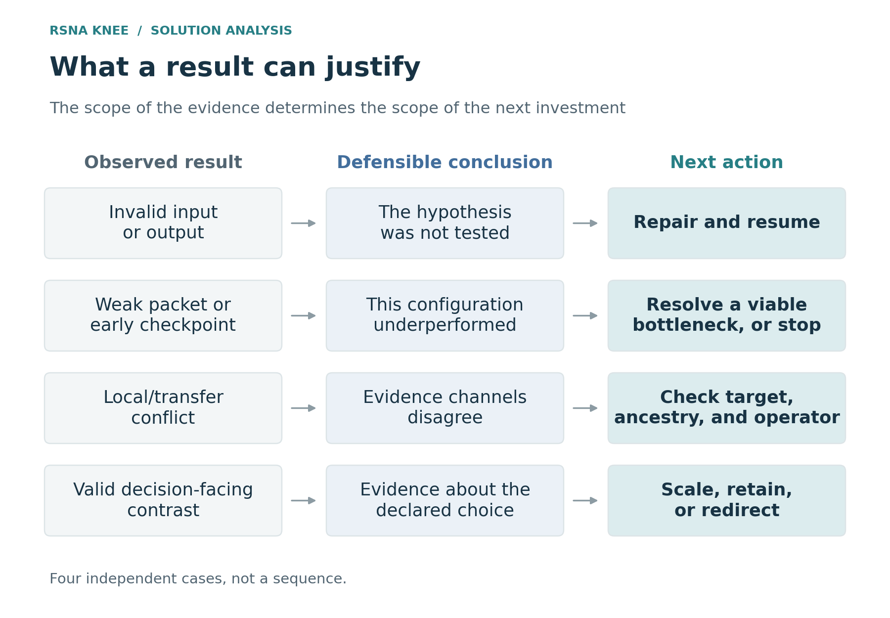
Figure 10. These are different types of evidence, not successive stages that every experiment must pass. A broader claim requires the corresponding comparison; a viable unresolved bottleneck may justify another test, while excessive cost or a failed necessary condition may justify stopping.

Invalid input or output calls for repair and resumption of valid completed work. A compatible full comparison with no benefit normally reduces or redirects the branch unless a specific unresolved mechanism justifies another test. Limited evidence requires naming what remains unidentified and deciding whether resolving it is worth the cost. A local/transfer conflict requires investigation of the mismatch, not a universal winner among metrics.

Positive evidence also has a scope. It may justify one complete family, a replacement at the same runtime, or one declared Public comparison. It does not automatically fund every architecture, target blend, and seed near the winner. Expansion should follow the supported mechanism, retaining enough control to detect a gain that disappears in the next setting.

An experiment record that changes the next decision

A short record is enough if it makes the next choice explicit.

Decision item	Concrete question before spending	What would change the next action?
Bottleneck	Which error or missing capability limits the current predictor?	Evidence that a different mechanism is responsible
Intervention and control	What changes, what stays fixed, and what does the learner actually receive?	A matched contrast at the level of the hypothesis
Evaluation	Which target, cases, group exclusions, and prior feedback support the comparison?	A demonstrated reference or deployment mismatch
Full price	What must finish before this becomes a selectable prediction?	Readiness, critical-path time, and the option displaced
Outcome branches	What happens after a positive, negative, invalid, or unresolved result?	A different experiment, allocation, or final choice

The record should change with the hypothesis, not become a new grand programme after every score. If every outcome leads to the same next run, the experiment may serve a stated diagnostic or learning goal, but contributes little to immediate selection. Naming that purpose prevents routine exploration from becoming apparent evidence for the incumbent.

Target order, split exclusions, input identity, and declared inference behavior deserve checks because an error can invalidate the comparison. Repeating a completed check without a new failure mode supplies no new prediction information. Audit count should not replace run count as the next proxy for progress.

Reallocation as evidence accumulates

Three functions need to coexist: a valid current predictor, a serious attempt to change its limiting mechanism, and the diagnosis needed to interpret that attempt. Their allocation depends on bottlenecks and readiness, not a universal percentage. One long coherent training programme may deserve most compute; at another point, a small annotation study may be the most useful preparation for it.

Research stages should turn on evidence rather than fixed weeks. A working baseline permits questions about target and view adequacy. A useful coherent alternative warrants complete OOF and a parent-specific contribution test. Saturating descendants warrant moving the next major investment to another source or mechanism while preserving the bank. A useful public release requires a role and full reproduction or integration price, not another catalogue of forks.

Warnings then need operational consequences. A weak standalone frontier calls for a credible stronger recipe; repeated reference reversals restrict the selector’s scope; a strong student with little parent gain raises replacement, compression, or residual-error questions before more distillation. These conditions do not require every candidate to beat the comparator standalone. They specify what new capability would justify its cost.

Near the deadline, the priority becomes which ready option can still alter the final choice. A scored fallback protects worthwhile late attempts without paying their preparation, troubleshooting, collection, or selection costs. Backward scheduling starts from usable output and a decision, including platform waiting—not the last mathematical execution start. A timeout ends that delivery attempt; redesign requires a newly declared comparison.

The next experiment should address the failure the current evidence identifies. Missing target information, an inadequate view, and a misleading reference call for different interventions. My OOF assets provided a valid starting point for those comparisons; preserving them did not require funding another similar descendant.

Original sources and comparison scope

The sources describe different development paths. Label-table evaluations, matched student experiments, component knockouts, package submissions, and post-deadline probes support different conclusions. The notebook and classifier links identify the implementations used to check the operators.

1. RB & Matheus & Tucker & Tony, 5th-place solution. Report-label semantics, fold-excluded calibration, and matched versus coupled improvements. ↩︎ ↩︎² ↩︎³ ↩︎⁴ ↩︎⁵ ↩︎⁶ ↩︎⁷ ↩︎⁸ ↩︎⁹

2. RSNA hosts, Competition annotation guidance. Positive criteria are competition definitions, rather than a general clinical diagnostic rule. ↩︎

3. MURAD, 2nd-place solution. Report omissions, full-image reading, target-specific witness choices, and failed blind-read escalation. ↩︎ ↩︎² ↩︎³ ↩︎⁴ ↩︎⁵ ↩︎⁶ ↩︎⁷ ↩︎⁸ ↩︎⁹ ↩︎¹⁰

4. Barry, 7th-place solution with no external training data. Three-read protocol and finding-specific overcalling. ↩︎ ↩︎² ↩︎³ ↩︎⁴

5. joinT fusion, 8th-place solution. Image-first discrepancy review and finding-specific supervision mixtures. ↩︎ ↩︎² ↩︎³ ↩︎⁴

6. Driz Lo, 21st-place solution. Full-series viewer, probability diagnostics, and fixed-epoch student comparisons. ↩︎ ↩︎² ↩︎³ ↩︎⁴ ↩︎⁵ ↩︎⁶ ↩︎⁷

7. matsurih, 22nd-place solution. Metadata-supported image montages, image-primary framing, and task-specific labels. ↩︎ ↩︎² ↩︎³ ↩︎⁴ ↩︎⁵ ↩︎⁶ ↩︎⁷ ↩︎⁸ ↩︎⁹ ↩︎¹⁰

8. sakaku, 1st-place solution: better labels, anatomy-aware MRI models. The additional account belongs to the same winning team. Matched CoAt comparison, bounded reader, continuous outputs, and Mix5. ↩︎ ↩︎² ↩︎³ ↩︎⁴ ↩︎⁵ ↩︎⁶ ↩︎⁷ ↩︎⁸

9. Honda Gen-AI EXPs, 32nd-place solution. Targeted replacement of 847 report/image-disagreement cells, not a global image-weight ablation. ↩︎ ↩︎² ↩︎³ ↩︎⁴ ↩︎⁵

10. chengtingyi, Astra Is All You Need?. Target-specific contact sheets, blind-reader complementarity, prompt-reference exposure, and annotation-budget comparisons. ↩︎

11. Amanie El-Hajj, 74th-place solution. Finding-specific reader acceptance and sensitivity to crop/zoom. ↩︎ ↩︎² ↩︎³ ↩︎⁴ ↩︎⁵ ↩︎⁶

12. Civitasmass, Multimodal LLM relabeling and OOF self-distillation. Simple multimodal versus multi-step reading comparison. ↩︎ ↩︎²

13. 129th-place solution. A failed direct-image reader and report-rubric alternative. ↩︎ ↩︎²

14. tascj, 1st-place solution. Probability diagnostics and trained-guide comparisons. ↩︎ ↩︎² ↩︎³ ↩︎⁴

15. the fault in our stars, The Hospital Is a Variable Too. Report-group expert rates, level corrections, and counter-tests. ↩︎ ↩︎² ↩︎³

16. Komil Parmar, 49th-place solution. Reader/schema and report-information limitations; see the solution’s label section for the specific local-reader comparisons. ↩︎ ↩︎² ↩︎³ ↩︎⁴

17. 102nd-place solution. Twenty report responses per study and explicit missing-label rules. ↩︎

18. menphim, 72nd-place solution. Site-bias interventions, pooled/within-site evaluation, and extra report-reader comparisons. ↩︎ ↩︎² ↩︎³ ↩︎⁴ ↩︎⁵

19. 977th-place solution. The OAI experiment used radiograph-derived partial supervision, not the same supervision as the MOAKS-head examples. ↩︎ ↩︎² ↩︎³

20. tascj, Box-pooling classifier source, with first-place account. Pooling operation and auxiliary-head handling were checked in archived code. ↩︎ ↩︎²

21. tascj, Final inference notebook. The archived integration averages the two branches 1:1; checkpoint and run-group counts differ. ↩︎

22. MURAD, pinned model source and knee-centre/local-view source. Static inspection of the post-competition rewrite, not a rerun of the original submission. ↩︎

23. Volkopat, 73rd-place KneeSplatNet account. Distinguishes the staged reader, the geometric prototype and its same-checkpoint knockouts, and the actual selected 2.5D model ensemble. ↩︎

24. 63rd-place solution. The SSL and partial-supervision comparisons were specific to the author’s models and reference panels. ↩︎ ↩︎² ↩︎³

25. tascj, Efficiency inference notebook. The 1,200-study preparation branch and packaged TensorRT route were inspected in the archived source. ↩︎

26. hirokenn, 33rd-place silver solution. Training-only trap, inference-only intervention, acquisition prediction, and controlled progression. ↩︎ ↩︎²

27. Akhyar Ahmad, 228th-place report-style prior subtraction. Metadata-only prior, sign probes, and the P7/P25 reversal. ↩︎ ↩︎²

28. 246th-place report labels and expert labels. OA coupling, report-reference reversal, and independent OAI checks. ↩︎ ↩︎²

29. Prahas Duggireddy, Own models on radiology reports. First-round gains, later plateaus, and explicit teacher-induced evaluation contamination. ↩︎ ↩︎²

30. 76th-place RSNA Knee AI solution. Gold-tuned teachers, repeated generations, matched failures, and inherited supervision. ↩︎

31. Mikkel Chávez Petersen, 302nd-place solution. The text reports eighteen own models and standardized-logit averaging; it does not provide a component ablation table. ↩︎ ↩︎²

32. Jay Gautam, 499th-place solution. Deployed-chain replay on 104 studies, gold checkpoint-selection exposure, split-half selection rules, and S6 weights. Split repetitions are not additional independent expert cases. ↩︎

33. M. Ehtasham, 412th-place solution. The S6 outer-arm comparisons, inherited finding weights, and final-stage fallback behavior. ↩︎ ↩︎²

34. Northstar, 65-submission postmortem. S6 placement, own-arm limitations, and the original-versus-fine-tuned CoAtNet inference control. ↩︎ ↩︎²

35. yu_kuo14, 507th-place solution. Full-chain gold evaluation with explicit upstream and repeated-selection exposure. ↩︎

36. Chris Deotte, 243rd-place solution. Hybrid annotations and the stated 2D-allocation blend while retaining the public 3D component. ↩︎

37. Robson, 215th-place field-strength rank correction. The reported Public correction sequence is separate from the final package Private score. ↩︎

38. Semyon Davshits and Ivan Safonov, 220th-place solution. One-epoch gold-batch fine-tunes, parameter soups, and the final multi-reader package. ↩︎

39. Shivoo29, 348th-place solution. Separates its selected public mixture from later self-training results and an external-pretraining route it declined to submit. ↩︎