BioHub Cell Tracking Working Note 2: From a Leaderboard Plateau to OOF Structural Diagnostics

Series links and references

• Competition: BioHub - Cell Tracking During Development
• Official metric notes: RoyerLab kaggle-cell-tracking-competition metrics.md
• Previous note: BioHub Cell Tracking Working Note 1: Learned Lineage Graphs and Metric-Aware Repair

• Korean version: BioHub Cell Tracking 작업 기록 2: Public 점수가 멈췄을 때 — OOF 기반 오류 분석

• Follow-up: BioHub Cell Tracking Working Note 3: What the OOF Machine Refused

Related public notebooks

• Biohub Cell Tracking: Data Model, EDA, Baseline
• Biohub Cell Tracking: Learned Graph w Gap Recovery
• Biohub Cell Tracking: Blend Preprocessings

About this series. BioHub asks competitors to reconstruct cell lineage graphs from 3D microscopy movies. The labeled training set contains 199 movies from two embryos; Public scores cover 29% of the hidden test set, and Private scores cover the remaining 71%. The hidden test comes from embryos not seen in training. Each note follows the record through its stated period; later findings and retrospective comments are marked separately.

Later context — September 23, 2026. On July 18 the division metric was patched, and the announced rescore later moved the leading Public score from about 0.970 to about 0.942. The ±0.002 Public tie rule used here was adopted on September 5–6.

Note 1 ended by asking which structural errors could be corrected on an unseen embryo. The recalibrated UNET400 anchor had reached about \(0.902\) on Public, but further checkpoint, threshold and blend variants gave little separation. Most inherited the anchor’s downstream calibration, so this plateau could not distinguish correlated model errors from calibration mismatch.

The next question was more concrete: which graph edits recover a real error, and does their net benefit survive on a held-out embryo? This note sets out an out-of-fold (OOF) design: each movie is predicted by a model trained without it, and the resulting graphs supply structural diagnostics. Training was still running on July 14, so the evaluations described here were a plan.

---

0. What Changed After the First Note

Until the first note, most gains followed this sequence:

learned node and edge scores
-> ILP base graph
-> motion relinking
-> short-component pruning
-> conservative gap and division repair

I then explored checkpoints, detection thresholds, TTA, center conditions, and mixtures with an independently seeded model. Representative public results were:

experiment family	representative score	observation
calibrated UNET400 motion and division graph	0.902	working anchor; within 0.001 of conditional Center
Center confirmation only for ambiguous gaps	0.901	a narrow confirmation rule; no resolved gain over the anchor.
broad Center validation of every synthetic gap	0.898	0.003 below conditional confirmation; useful repairs may have been vetoed.
detection-threshold brackets	0.899	the tested threshold brackets did not beat the anchor.
shared-point association TTA	0.899–0.900	the tested TTA settings did not improve the calibrated graph.
fixed-ratio independent-seed blends	about 0.901	the tested ratios did not beat the anchor.
low-margin seed consensus	about 0.901	the tested conditional gate did not expose a clear gain.

Public scores are rounded to three decimals. These readings narrowed the settings worth further testing, but small differences did not establish an ordering on new embryos.

At the time, the visible leaders scored \(0.970\) and \(0.968\), followed by \(0.941\) and \(0.938\). That gap motivated a broader search, but the scores alone could not locate the difference in detection, association or metric behavior.

---

1. A Checkpoint and Its Post-Processing Form One Model

Write the complete submission pipeline as

\[\hat G = P_{\theta} \left( M_W(X) \right).\]

Here,

• \(X\) is a 3D time-lapse sequence,
• \(M_W\) is the Temporal UNet and edge transformer with weights \(W\),
• \(P_\theta\) is ILP and deterministic graph processing with parameters \(\theta\), and
• \(\hat G\) is the submitted graph.

The vector \(\theta\) contains much more than one scalar threshold:

\[\theta= \left[ \tau_{\mathrm{det}}, \tau_{\mathrm{edge}}, \lambda_{\mathrm{motion}}, \lambda_{\mathrm{ILP}}, L_{\min}, C_{\mathrm{gap}}, C_{\mathrm{division}}, \ldots \right].\]

Longer training changes the distributions of both detection and edge logits. Even with the same visible threshold, it changes candidate counts, rankings, ILP choices, and the population seen by later repair stages. The following are therefore different systems:

UNET300 + theta_300
UNET400 + theta_300

The second line is not simply a better-trained version of the first. It may be a 400-epoch checkpoint with a mismatched 300-epoch calibration.

This is one possible explanation for the score drops after a checkpoint change and the recovery after recalibration between 250 and 400 epochs; the submitted comparisons did not isolate calibration from checkpoint quality. A lower training loss and a better final graph are not the same optimization axis.

---

1.1 A Failed Fixed Blend Does Not Prove That Blending Has No Headroom

Let \(f_A\) be the anchor, \(f_B\) an auxiliary predictor, \(g_\alpha\) their combination, and \(\theta\) the complete downstream parameter vector. Repeated public-leaderboard iteration had approximately selected an anchor operating point \(\theta_A^*\).

Most completed blend experiments measured

\[S_{\mathrm{LB}} \left( g_{\alpha_0}(f_A,f_B), \theta_A^* \right),\]

or a small neighborhood around it. Failing to beat the anchor at that point does not imply

\[\max_{\alpha,\theta} S\left(g_\alpha(f_A,f_B),\theta\right) \le \max_{\theta} S\left(f_A,\theta\right).\]

The distinction is clearer when the two questions are written separately:

\[\Delta_{\mathrm{fixed}} = S_{\mathrm{OOF}}\left(g_{\alpha_0},\theta_A^*\right) - S_{\mathrm{OOF}}\left(f_A,\theta_A^*\right),\] \[\Delta_{\mathrm{joint}}^* = \max_{\alpha,\theta} S_{\mathrm{OOF}}\left(g_\alpha,\theta\right) - \max_{\theta} S_{\mathrm{OOF}}\left(f_A,\theta\right).\]

The submitted experiments gave a noisy public-leaderboard proxy for \(\Delta_{\mathrm{fixed}}\). Even if \(\Delta_{\mathrm{fixed}}\le0\), it does not follow that the jointly calibrated headroom \(\Delta_{\mathrm{joint}}^*\) is non-positive.

A blend changes all of the following distributions:

1. absolute detection-logit scale,
2. edge-candidate ranking and margins,
3. node count per frame,
4. costs competing inside the ILP,
5. inputs to motion reassignment, and
6. the candidate populations for gap and division repair.

The best downstream operating point may therefore move from \(\theta_A^*\) to a different \(\theta_{\mathrm{blend}}^*\).

1.2 Three Explanations That the Public Scores Cannot Separate

The fixed-blend results are compatible with at least three hypotheses:

hypothesis	meaning
high error correlation	The auxiliary model fails where the anchor fails.
calibration mismatch	Unique useful evidence exists, but \(\theta_A^*\) is wrong for the combined distribution.
Public-LB adaptation	Repeated submissions adapted \(\theta_A^*\) too closely to the visible subset.

The existing Public scores cannot identify which explanation dominates. The precise conclusion is therefore:

The tested fixed blends and conditional gates did not beat the anchor
under the inherited downstream calibration.

The globally attainable optimum of a jointly calibrated blend remains unknown.

Large-scale joint tuning directly against the Public leaderboard would not solve the inference problem. It could simply deepen adaptation to the visible subset. Joint calibration must instead be measured on predictions from videos that were not used to fit the underlying models.

---

2. The Errors Defined by the Official Metric

Note 1 introduced the score. The diagnostics planned here depend on three details: which false edges count under sparse annotation, how node counts affect the score, and how the July 14 scorer recognizes a division.

2.1 Edge Jaccard Under Sparse Annotation

Predicted and ground-truth nodes are paired within the same frame by optimal bipartite matching, with a maximum physical distance of \(7\,\mu\mathrm{m}\). A predicted edge is a true positive when both endpoints match ground-truth nodes joined by a ground-truth edge.

\[J_{\mathrm{edge}} = \frac{TP}{TP+FP+FN}.\]

Because labels are sparse, not every unmatched predicted edge is an FP. Only edges that can be shown to be wrong inside annotated context are penalized. Raw node and edge counts are therefore insufficient for diagnosing a change.

2.2 Node-Count Adjustment

For sample \(i\), let \(N_{\mathrm{pred},i}\) be the predicted-node count and \(N_{\mathrm{total},i}\) the supplied coarse estimate of all cells. Define

\[r_i = \frac{N_{\mathrm{pred},i}-N_{\mathrm{total},i}} {N_{\mathrm{total},i}}.\]

The adjusted edge score is

\[J_{\mathrm{adj},i} = \max \left( 0, J_{\mathrm{edge},i}(1-0.1r_i) \right).\]

The aggregate edge score is not an unweighted mean over videos. It uses \(D_i=TP_i+FP_i+FN_i\) as the sample weight:

\[J_{\mathrm{edge}}^{\mathrm{adjusted}} = \frac{\sum_iD_iJ_{\mathrm{adj},i}} {\sum_iD_i}.\]

When \(r_i<0\), the multiplier can exceed one. That is not an invitation to underpredict nodes: removing nodes can first increase edge FNs and damage the unadjusted Jaccard. The implication is that detection and association cannot be optimized independently.

2.3 Division Scoring Is Broader Than a Direct Parent-to-Two-Children Match

This section describes the metric in force on July 14.

The final score is

\[S = J_{\mathrm{edge}}^{\mathrm{adjusted}} +0.1J_{\mathrm{division}}.\]

Division Jaccard is also micro-averaged over all events rather than averaged over per-video ratios:

\[J_{\mathrm{division}} = \frac{\sum_iTP_i^{\mathrm{div}}} {\sum_i\left(TP_i^{\mathrm{div}}+FP_i^{\mathrm{div}}+FN_i^{\mathrm{div}}\right)}.\]

The official division condition is more structural than I initially assumed. A ground-truth division is recovered when one weakly connected predicted component

1. contains a matched pre-division-stage node,
2. touches both daughter lineages,
3. connects those stages in one component, and
4. contains a predicted fork with out-degree two.

The predicted fork need not be a node directly matched to the exact ground-truth divider at the exact split time. An unmatched intermediate fork can still complete the required lineage topology.

This changes division recovery from “add a second edge next to the matched parent” into:

Connect the pre-stage and both daughter lineages in one component,
while adding as few harmful edges and nodes as possible.

---

3. What the Experiments Established

3.1 What the 300-Epoch versus 400-Epoch Comparison Showed

Applying both all-train models back to the same 199 training videos favored the 400-epoch checkpoint:

metric	UNET300	UNET400	delta
edge TP	121,669	122,151	+482
edge FP	5,212	5,202	-10
edge FN	7,214	6,732	-482
global edge-Jaccard proxy	0.907334	0.910997	+0.003663
mean score proxy	0.902110	0.912574	+0.010464

The error reasons also showed that UNET400 did more than increase confidence:

error reason	UNET300	UNET400	interpretation
missing edge between matched nodes	5,535	5,384	fewer association misses
source-node-unmatched FN	710	548	better node matching
target-node-unmatched FN	709	579	better node matching
both-nodes-unmatched FN	260	221	fewer sparse detection failures

These counts described how errors changed between all-train checkpoints. They helped design repair candidates around the UNET400 anchor already chosen through Public comparisons; accepting a new policy or validating a checkpoint choice required held-out predictions.

---

3.2 Why I Stopped Spending Submissions on Parameter Perturbations

The following axes had already been explored around the plateau:

detection threshold
minimum track length
gap distance and cap
division geometry
Center threshold
TTA aggregation
independent-seed blend ratio
low-margin consensus gate

Those experiments were useful. They mapped local sensitivity and showed several unsafe directions. The problem was the declining information returned by each new submission.

Suppose a fixed blend scores \(0.901\). The single public number cannot tell us whether

1. the auxiliary model contributes almost no unique correct edges,
2. unique correct edges were diluted by averaging,
3. logit miscalibration caused the ILP to choose the wrong candidates,
4. edge quality improved while node adjustment or division quality declined, or
5. the difference is hidden by rounding.

One more blend ratio does not resolve these explanations. An OOF candidate table can expose TP, FP, FN changes and stability by video directly.

Stopping parameter sweeps therefore does not mean that every parameter is globally optimized. It is a resource-allocation decision: do not continue one-axis Public-LB search without new held-out evidence.

---

4. Designing Strict OOF

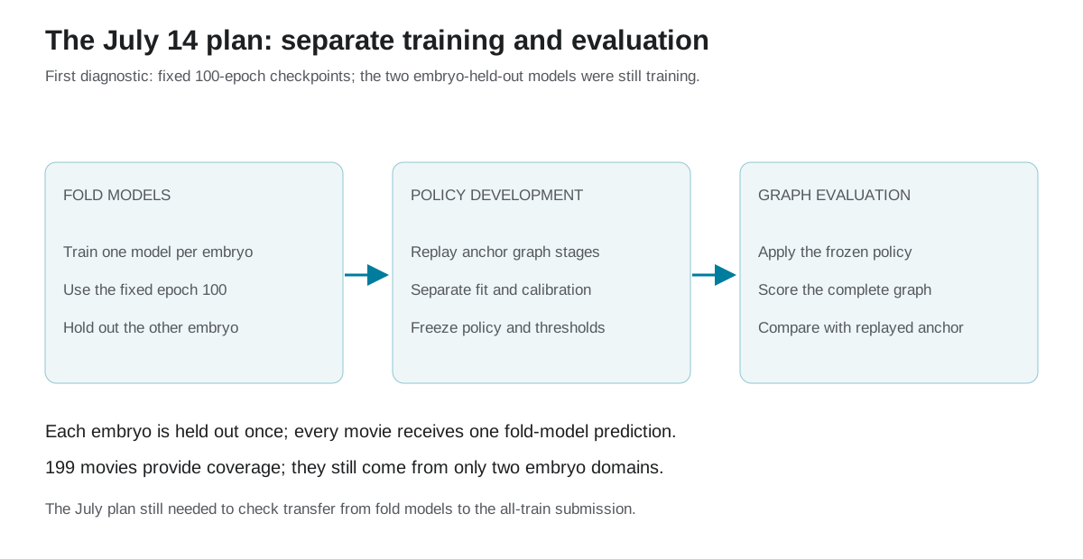Figure 1. The July validation plan: generate predictions from fixed-epoch fold models, separate policy fitting, calibration and evaluation, and compare complete graphs. The held-out embryo must stay out of every training and selection step.

An OOF prediction for sample \(i\) must come from a model that did not train on that sample:

\[\hat G_i^{\mathrm{OOF}} = P_{\theta_0} \left( M_{W_{-k(i)}}(X_i) \right),\]

where \(W_{-k(i)}\) was fitted without fold \(k(i)\). The current twofold split keeps embryo families disjoint. Each model predicts only its own holdout, and every training video must appear exactly once in the merged OOF set.

Producing OOF predictions does not by itself make policy selection unbiased. The data used to fit a repair policy, calibrate its threshold, and report its final gain must also have separate roles:

\[\mathcal D_{\mathrm{fit}}\cap\mathcal D_{\mathrm{cal}} = \mathcal D_{\mathrm{fit}}\cap\mathcal D_{\mathrm{eval}} = \mathcal D_{\mathrm{cal}}\cap\mathcal D_{\mathrm{eval}} = \varnothing,\] \[\phi^* = \arg\max_{\phi} S\left( \mathcal D_{\mathrm{cal}}; R_{\phi}(\hat G^{\mathrm{OOF}}) \right), \qquad \text{report } S\left( \mathcal D_{\mathrm{eval}}; R_{\phi^*}(\hat G^{\mathrm{OOF}}) \right).\]

Here \(\mathcal D_{\mathrm{fit}}\) trains the policy, \(\mathcal D_{\mathrm{cal}}\) chooses operating thresholds, and \(\mathcal D_{\mathrm{eval}}\) supports the final claim. With limited data, cross-validation can rotate fitting and calibration inside outer training. There are still only two independent embryo domains. The fixed-epoch design below addresses checkpoint selection; keeping policy development separate from evaluation also requires the data roles above.

Code: minimum OOF coverage checks

from collections import Counter

coverage = Counter()

for fold in folds:
    train_ids = set(split[fold]["train"])
    holdout_ids = set(split[fold]["test"])

    assert train_ids.isdisjoint(holdout_ids)
    assert {embryo_of[m] for m in train_ids}.isdisjoint(
        {embryo_of[m] for m in holdout_ids}
    )

    predictions = predict(
        model=fold_models[fold],
        datasets=sorted(holdout_ids),
    )
    coverage.update(predictions.keys())

assert set(coverage) == set(all_training_ids)
assert all(count == 1 for count in coverage.values())

4.1 Selecting the Best Epoch on the Outer Holdout Is Leakage

The first capture design contained an important flaw. It planned to use edge_predictor_best.pth, saved at the epoch with the best outer-holdout score, to predict that same outer holdout. The samples were not used for gradient updates, but they were used for epoch selection.

Formally, it selected

\[e^* = \arg\max_e S_{\mathrm{outer}} \left(W_e\right)\]

and then reported \(S_{\mathrm{outer}}(W_{e^*})\) on the same data. That is not a fixed OOF estimate.

The corrected contract is:

precommit 100 epochs as the first diagnostic checkpoint
use checkpoint_last.pth@100 for each fold
verify fold, method, split, and epoch from the manifest
never use the outer holdout to choose the best checkpoint

The 100-epoch checkpoint is not claimed to be the final performance optimum. It is a precommitted point for diagnosing event types and generating policy candidates.

4.2 Extending to 200 Epochs

Selecting 200 epochs after seeing that it scores better on the same outer holdout would reintroduce selection leakage. There are two valid approaches:

1. precommit 200 epochs before inspecting the relevant outer-holdout results, or
2. create an inner validation split inside each outer-training fold and select the epoch only on that inner split.

Captures must remain separate, for example ep_0100 and ep_0200. Later checkpoints must not overwrite the earlier decision record.

---

4.3 Raw OOF Is Not Submission-Graph OOF

The Temporal UNet and transformer output is not the final submitted graph. The anchor notebook applies deterministic stages afterward:

raw model graph
-> ILP selection
-> motion reassignment
-> short-component pruning
-> one-frame gap recovery
-> safe division repair
-> submission graph

Raw fold predictions are useful for model anatomy, but do not evaluate the complete \(0.902\) notebook. Its motion, pruning, gap and division stages must also be replayed. Matching those stages is necessary; independent checkpoint and policy selection are still needed for an unbiased estimate.

This is part of the evaluation contract, not optional implementation polish.

4.4 Fixed Inference Operating Point

The raw capture is pinned to an operating point aligned with the anchor’s node distribution:

item	value
detection threshold	0.9700
detection TTA	XY D4
edge-feature TTA	original feature map
pooling kernel	\(3.0\,\mu\mathrm{m}\)
edge activation	softmax
edge threshold	0.5
ILP	enabled
association learned-edge bonus	1.0

This is the current replay anchor. Note 1 illustrated an earlier association bonus of \(0.75\); here it is \(1.0\). The \(0.901\) Center configuration and the \(0.902\) anchor also differ as complete packages, so their displayed difference does not isolate that bonus.

Every capture must record:

fold id
train/holdout split hash
weight SHA256
checkpoint epoch
method name
inference profile
prediction dataset list

A filename or directory name is not a sufficient model identity once many seeds, folds, and checkpoints coexist.

---

5. Decomposing OOF Errors into Structural Events

The first readout after capture should not be one global score. I plan to inspect, in order:

1. predicted-node ratio by sample,
2. edge TP, FP, FN and raw versus adjusted Jaccard,
3. division TP, FP, FN,
4. deltas by embryo family,
5. sign and magnitude of per-video deltas, and
6. counterfactual score changes for each candidate edit.

5.1 Structural Classes for Division FNs

Each missed ground-truth division can be assigned to one structural class:

class	meaning	appropriate intervention
connected_without_fork	Required stages share a component, but it has no fork.	bounded second outgoing edge
stages_disconnected	Necessary nodes exist but lineage stages are disconnected.	scored bridge-plus-fork candidate
missing_pre_stage	No pre-division detection is available.	detection model or Center feature
missing_daughter_lineage	One daughter lineage is absent.	improve detection; do not force a graph-only repair
fork_assignment_conflict	A fork exists but corresponds to a different event.	event-level assignment model
no_matched_nodes	No safe topological evidence is available.	no intervention

The classes matter because one operator cannot safely repair all division FNs. A single extra edge may solve connected_without_fork, while applying it to missing_daughter_lineage would mostly create FPs.

5.2 The Actual Objective for a Repair Operator

The value of an operator \(R\) is not the number of recovered true edges alone:

\[\Delta S_R = \Delta J_{\mathrm{edge}}^{\mathrm{adjusted}} +0.1\Delta J_{\mathrm{division}}.\]

Recovering one division while adding several harmful edges or distorting node count can lower the combined score. Conversely, one carefully placed fork can complete several structural division conditions at a small edge cost.

Graph edits are generally non-additive:

\[\Delta S(R_1\cup R_2) \ne \Delta S(R_1)+\Delta S(R_2).\]

Two edits can alter the same connected component, division event, or Jaccard denominator. The final policy must therefore rescore the selected edit set, including ordering and interactions, with the official metric.

---

6. Graph Policies to Test with OOF

6.1 Conservative Edge Replacement

Rebuilding every edge in the anchor graph would have a large blast radius. The first policy is restricted to changing the target of an existing next-frame association.

For source \(i\), let \(G_i\) be its next-frame candidate group and \(s_{ij}\) the ranker score for candidate \(j\). A group-wise objective is

\[\mathcal L_i = \log\sum_{j\in G_i}\exp(s_{ij}) - \log\sum_{j\in G_i:y_{ij}=1}\exp(s_{ij}).\]

The feature vector uses quantities directly related to the observed errors:

\[x_{ij}= \left[ p_{ij}, d_{\mathrm{raw}}, d_{\mathrm{motion}}, \operatorname{rank}_{ij}, |G_i|, \deg^+(i), \deg^-(j), \rho_i, \rho_j, t_{\mathrm{norm}}, \ldots \right].\]

The anchor motion-assignment score can be written as the negative cost

\[A_{ij} = -\left( d_{\mathrm{motion}} +0.05d_{\mathrm{raw}} -1.0p_{ij} \right).\]

For the ranker target \(r\) and anchor target \(a\), define

\[\Delta s=s_{ir}-s_{ia},\] \[\Delta A=\max(0,A_{ia}-A_{ir}).\]

A replacement is enabled only if OOF calibration passes benefit precision, harmful-change rate, edit-count, and per-video stability requirements.

Code: conservative, non-cascading replacement

def can_replace(proposal, graph, frozen_claims, policy):
    source = proposal.source
    current = proposal.current_target
    alternative = proposal.alternative_target

    if graph.out_degree(source) != 1:
        return False
    if graph.in_degree(current) != 1:
        return False
    if alternative in frozen_claims:
        return False
    if proposal.rank_margin < policy.min_rank_margin:
        return False
    if proposal.anchor_penalty > policy.max_anchor_penalty:
        return False
    return True

The policy cannot

• add nodes,
• create divisions,
• steal an already claimed target,
• use one replacement as input to a later replacement, or
• force itself on when OOF calibration fails.

If no threshold set passes, the packaged policy remains enabled=false. Relaxing it manually just to create a submission would defeat the purpose of OOF.

---

6.2 Division-Event Recovery

If connected_without_fork dominates, the smallest useful operator is one extra outgoing edge. Candidate generation can require

the same or an adjacent tolerated division time
enough spatial separation between daughter candidates
motion compatibility with the parent
continuation evidence for both daughters
valid in-degree and out-degree constraints
per-video and per-graph edit caps

If stages_disconnected dominates, the policy must evaluate a bridge and a fork together. That has a higher edge-FP risk and should not be deployed as a fixed distance rule.

An event-level scorer can use

\[z_{p,d_1,d_2} = \left[ q_{p,d_1}, q_{p,d_2}, r_{\mathrm{motion},1}, r_{\mathrm{motion},2}, d(d_1,d_2), c_{d_1}, c_{d_2}, \rho_p, t_{\mathrm{norm}} \right],\]

where \(q\) is learned edge evidence, \(r_{\mathrm{motion}}\) a motion residual, \(d(d_1,d_2)\) daughter separation, and \(c\) optional OOF Center support.

\[P(y_{p,d_1,d_2}=1\mid z) = \sigma(h_\phi(z)).\]

The purpose is not to create more divisions. It is to select the smallest set of graph edits whose division gain exceeds their edge cost.

---

7. When Auxiliary Models Become Useful Again

7.1 Center Model

The Center model was unstable as a global node union or universal veto. It becomes relevant again if OOF anatomy shows substantial missing_pre_stage or missing_daughter_lineage mass.

The required feature is not an all-train Center score on its own training videos. It must be fold-held-out Center support for the same OOF events:

graph and motion evidence
+ held-out Center support
-> event-level decision

Low Center confidence should not reject a strong temporal candidate by itself. High Center confidence can support an event where graph evidence is otherwise marginal.

7.2 Independent Seeds and Blending

The value of an independent seed lies in events it gets uniquely right, not in its average score alone. Start with the four-way complementarity table:

anchor	auxiliary	meaning
correct	correct	safe agreement
correct	wrong	region where blending can damage the anchor
wrong	correct	the recoverable complementarity we need
wrong	wrong	unlikely to be solved by a simple ensemble

Define selector-oracle uplift as the score of an ideal event-wise selector minus the better individual model:

\[U_{\mathrm{oracle}} = S_{\mathrm{oracle}(A,B)} - \max(S_A,S_B).\]

An oracle over this fixed candidate set can show whether the models supply complementary correct events there. A small uplift limits that selector’s scope, not every possible blend. A large uplift motivates a selector or calibration experiment, but does not show that a deployable model can identify the oracle’s choices.

The next valid blend experiment is therefore

\[(\alpha^*,\theta^*) = \arg\max_{\alpha,\theta} S_{\mathrm{OOF}} \left( g_\alpha(f_A,f_B), \theta \right),\]

with another split between calibration and final evaluation.

---

8. Established Results, Working Hypotheses, and Open Questions

8.1 Established

1. One-axis sweeps around the current anchor calibration did not produce a material Public-LB gain.
2. The all-train 400-epoch model has better in-sample edge anatomy than the 300-epoch model.
3. The tested narrow Center confirmation scored above the broad-veto variant on Public; this was not an independent estimate of reliability.
4. The tested fixed TTA and independent-seed blends did not beat the anchor.
5. The official metric couples node count, edges, and division-component topology.

8.2 Working Hypotheses

1. After the scalar sweeps, testing a new graph decision rule was the more informative next experiment.
2. Event-level division recovery and conservative edge replacement may complement the anchor.
3. Auxiliary-model features for uncertain events were an alternative to the global averages already tested.
4. A jointly calibrated blend has not been ruled out.

8.3 Questions That Require Strict OOF

1. What is the held-out score after replaying the anchor-equivalent graph stages?
2. Which structural classes dominate division FNs?
3. Does the edge-replacement ranker provide net gain in both embryo families?
4. Does Center add information after conditioning on graph and motion features?
5. Is there meaningful selector-oracle uplift between independent seeds?
6. Are 100-epoch fold models trained enough to provide stable error labels?

Keeping these categories separate matters. Turning “plausible” into “established” would send the experiment loop back to leaderboard guessing.

---

9. Promotion Gates for an OOF Policy

A positive aggregate OOF point estimate is not enough. A graph-edit policy advances only if

1. the exact combined \(\Delta S\) is positive,
2. neither embryo family has a negative aggregate delta,
3. gains are distributed across videos rather than carried by one or two,
4. node adjustment is not hiding a large raw edge-Jaccard loss,
5. absolute and fractional edit counts are bounded,
6. feature generation and notebook runtime use identical coordinates, units, and candidate gates, and
7. epoch selection, policy fitting, threshold calibration, and final evaluation are separated where required.

Paired resampling by video gives a within-panel stability check. The example below resamples the unweighted mean of movie deltas; it is not the competition aggregate, which must be recomputed from edge denominators, node adjustments and pooled division counts in each draw. Neither version removes uncertainty from having only two embryos or from repeated selection on the same panel.

Code: movie-mean diagnostic, separate from official aggregation

import numpy as np

def paired_bootstrap(delta_by_video, repeats=5000, seed=2026):
    values = np.asarray(delta_by_video, dtype=float)
    rng = np.random.default_rng(seed)
    samples = rng.choice(values, size=(repeats, len(values)), replace=True)
    means = samples.mean(axis=1)
    return {
        "mean": float(values.mean()),
        "fraction_positive_draws": float((means > 0).mean()),
        "q025": float(np.quantile(means, 0.025)),
        "q975": float(np.quantile(means, 0.975)),
    }

---

10. Run Status on July 14 and the Planned Sequence

As of July 14, the OOF run was in progress under this contract:

method: twofold TemporalUNet3D + association transformer
seed: 271828
split: embryo-disjoint twofold
first diagnostic epoch: fixed 100
OOF weight: checkpoint_last.pth@100
outer-holdout best checkpoint: not used

Capture and analysis code was strengthened while training was running, but the training data, split, seed, loss, optimizer, augmentations, and target epoch did not change. The changes affect fixed-epoch verification and post-training prediction capture. There is therefore no reason to discard and restart the current run.

After both folds finish, the sequence is:

1. verify each fixed-epoch checkpoint
2. verify holdout coverage and weight hashes
3. capture raw OOF predictions
4. compute exact edge and division anatomy
5. replay the anchor's deterministic graph stages
6. evaluate edge-replacement and division-recovery candidates
7. check stability by embryo and video
8. transfer only passing policies to the all-train 400-epoch anchor

The 100-epoch fold models were intended to diagnose errors and screen policies, while the all-train model would produce final predictions. Transferring a policy between them still needed a check: changing model weights can change logits, selected nodes and repair candidates.

\[\text{OOF models} \rightarrow \text{policy selection},\] \[\text{all-train model} \rightarrow \text{final prediction}.\]

---

Closing

The repeated ties narrowed the settings worth testing further. The next step was to generate fixed-epoch fold predictions and compare complete graphs, with known error types, a fixed comparator, and separate fitting, calibration and evaluation roles. That would show which proposed repairs were worth carrying forward.

Series:

• 1: Learned Lineage Graphs and Metric-Aware Repair

• 2: From a Leaderboard Plateau to OOF Structural Diagnostics

• 3: What the OOF Machine Refused

• 4: Three Gaps in Local Validation

• 5: What a Frozen Graph Left Untested

• 6: When Local Validation Ran a Different Pipeline

• 7: When the Same Code Was Not the Same Experiment

• 8: What Went Into Choosing the Final Two