ROGII Competition Retrospective: A Silver Medal and Lessons from the Public-Private Gap

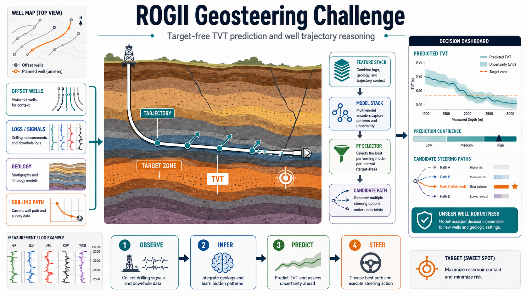
ROGII Competition Retrospective: A Silver Medal and Lessons from the Public-Private Gap

This is my final retrospective on the ROGII Wellbore Geology Prediction competition. The first two articles developed the problem formulation and decomposed the error. This one records how those ideas became a submission system, how the system evolved over two months, and what the final public/private shake-up revealed.

Earlier articles:

• Part 1: Leakage-Controlled TVT Recovery Through Target-Free Stratigraphic Alignment
• Part 2: Error Anatomy of Target-Free TVT Geosteering

Korean version:
ROGII 대회 회고: Silver Medal까지의 여정과 Public/Private 격차의 교훈

Key links:

• ROGII - Wellbore Geology Prediction
• Final notebook: ROGII Development & Tests
• Working Note: Target-Free TVT Geosteering
• Final leaderboard

---

The result first

I finished 210th with a silver medal.

Item	Result
Team public score / rank	5.952 / 67th
Team private score / rank	8.197 / 210th
Score gap, private minus public	+2.245
Submission determining the final score	PS3 bounded TCN dual structural
Personal records returned by the API	339
Records with both public and private scores	301

Because lower RMSE is better, the +2.245 gap was a large deterioration. It was not, however, an isolated failure.

• The median gap across 6,191 matched teams was +1.929.
• Only one public top-10 team remained in the private top 10.
• The overlap between the public and private top 25 was 11 teams.
• The median gap among the public top 100 was +2.213.
• Public winner shu01 moved from 4.608 to 6.653, finishing 28th.
• Private winner Ruby moved from public rank 31 at 5.648 to private rank 1 at 5.639.

My +2.245 gap was therefore close to the public top-100 median. The public leaderboard was not useless, but it was not a sufficiently stable coordinate for choosing the final ranking either.

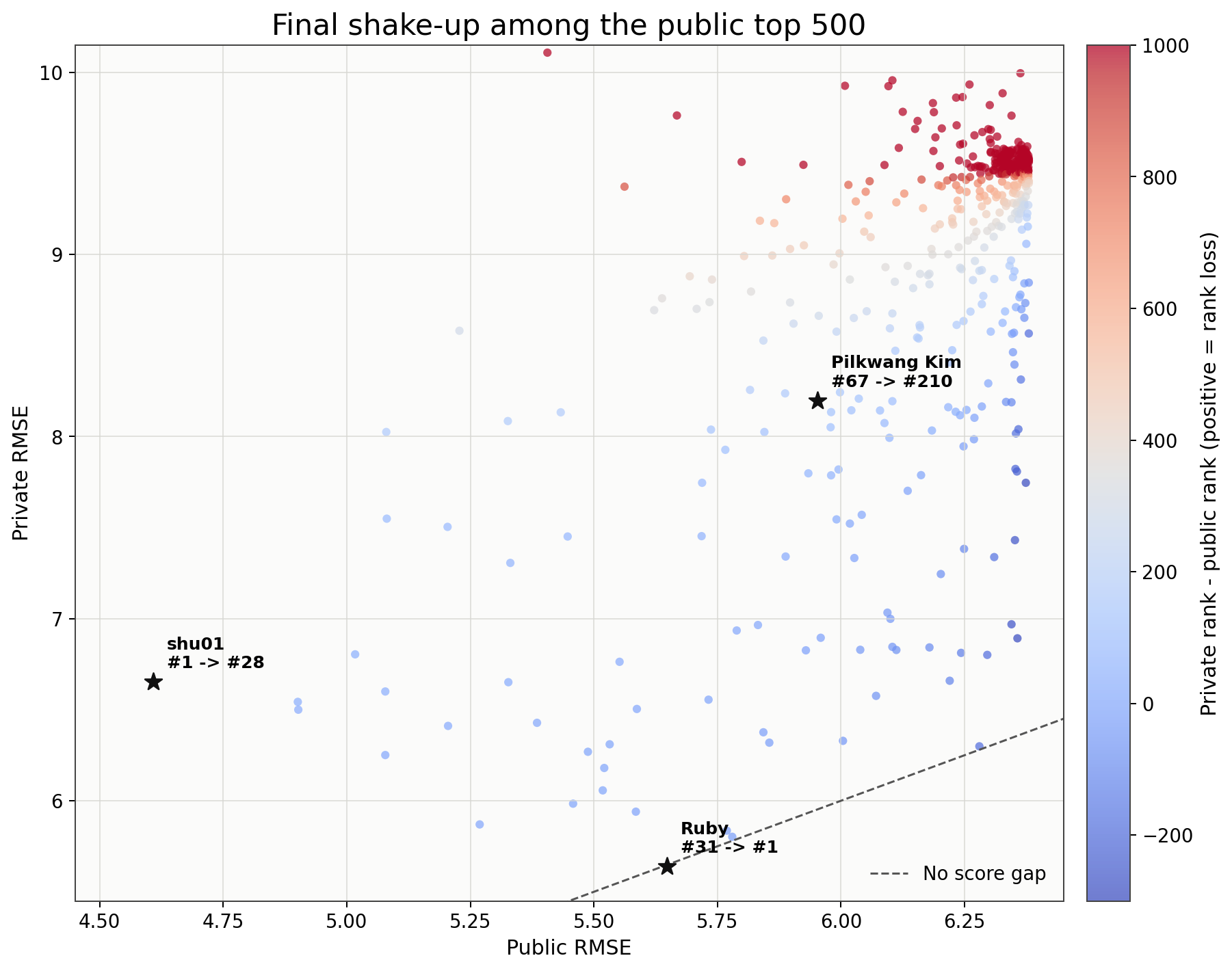
The figure matches the public top 500 to their final private scores. The dashed line is the no-gap diagonal, and color represents rank movement. Even near the top, both score gaps and rank reversals were substantial.

There is an important caveat. A team’s public leaderboard score can come from its best public submission, while its private score is determined by one of its selected final submissions. Team-level gaps therefore measure the standings shake-up, not always a pure distribution shift for one identical model. My submission-level analysis later in this article pairs the same submission reference and is the cleaner comparison.

---

Writing the problem in one equation

The task asked us to predict TVT over the hidden interval of a horizontal well. At first it looked like row-wise regression:

\[\widehat T_{w,i}=f(MD_{w,i},X_{w,i},Y_{w,i},Z_{w,i},GR_{w,i}).\]

But rows are not independent observations. Each row is a location along one continuous trajectory. The formulation I kept throughout the competition was:

\[\widehat T_w(s)=\widehat D_w+\widehat\phi_w(s), \qquad s\in[0,1].\]

Here:

• $\widehat D_w$ is the datum, which places the whole well inside the stratigraphic column;
• $\widehat\phi_w(s)$ is the shape of the hidden tail after that placement.

This representation changed the engineering. Instead of treating GR as one more feature, I aligned it to a typewell coordinate, used prefix TVT_input as an anchor, and treated repeated stratigraphic motifs as competing depth modes rather than forcing a hard argmin.

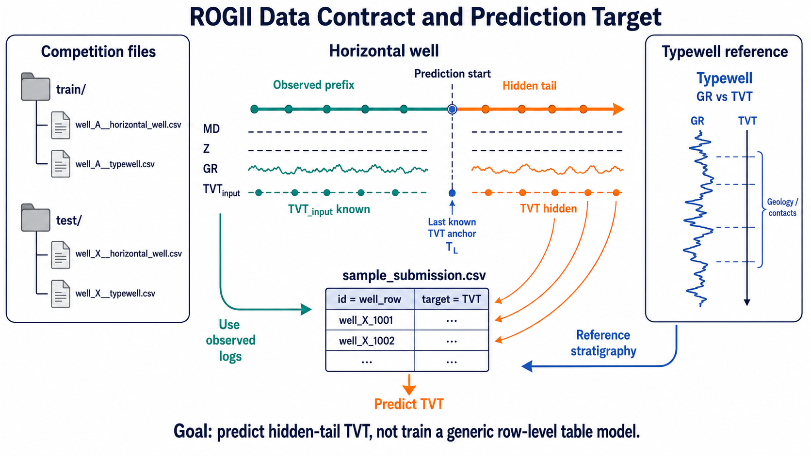
For well $w$, define the visible prefix and hidden tail as:

\[\mathcal P_w=\{i:T^{input}_{w,i}\ \text{is observed}\},\qquad \mathcal H_w=\{i:T^{input}_{w,i}\ \text{is missing}\}.\]

A valid estimator may use only:

\[\widehat T_{w,\mathcal H} =F\!\left( X_{w,\mathcal P\cup\mathcal H}, T^{input}_{w,\mathcal P}, \operatorname{typewell}_w \right).\]

The complete GR and trajectory traces are observed covariates in the test input and are therefore available. Hidden TVT, or any statistic derived from it, is not. This became the contract for every OOF matrix, feature builder, and runtime adapter.

---

Score progression: 8.336 ft on public, roughly 5.5 ft on private

My first public score was 14.288. The final public best was 5.952, an improvement of 8.336 ft.

The paired private scores tell a more nuanced story. The first submission scored 13.743 on private, while the selected final submission scored 8.197: a genuine improvement of 5.546 ft. It would therefore be wrong to say that the entire project was public overfitting. The structural improvements transferred, but a large fraction of the late public gain did not.

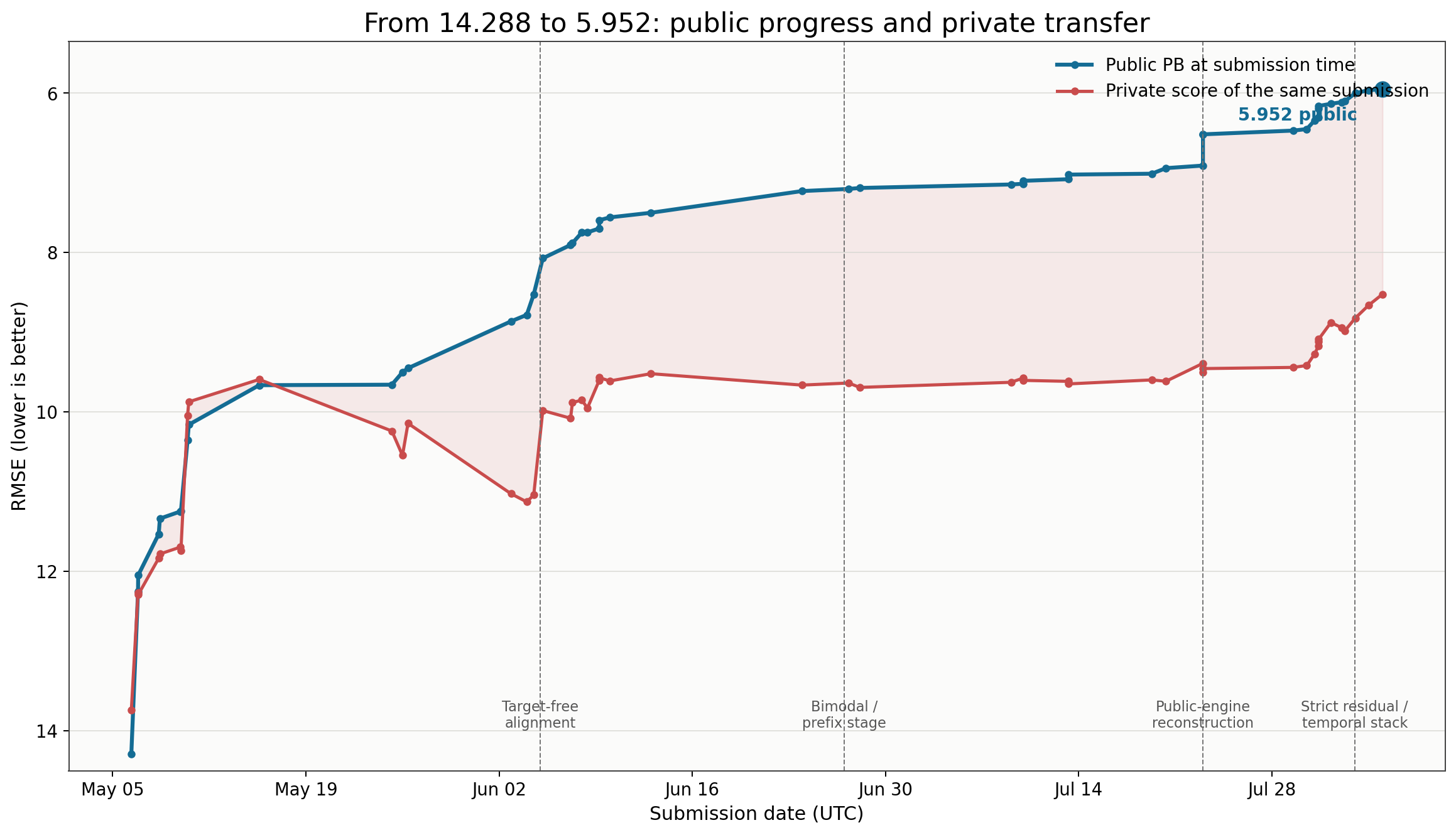
Representative public personal-best milestones were:

Date	Public	Private	Main change at the time
May 6	14.288	13.743	Initial EDA and residual modeling
May 10	10.160	9.873	Same-matrix model stack
June 5	8.072	9.982	Target-free alignment
June 8	7.747	9.952	Ridge/PF/projection composition
June 27	7.202	9.637	Visible-prefix and bimodal hedge
July 13	7.022	9.648	Dual-track prefix calibration
July 20	6.941	9.615	Seed-cloud datum branch
July 23	6.517	9.456	Source-complete public-engine reconstruction
July 31	6.161	9.088	Content-verified trajectory transfer
August 3	6.001	8.823	Query-temporal residual row
August 5	5.952	8.523	Bounded residual structural, PS1

The key discontinuity came in early June. Target-free alignment produced a large public gain, while private barely moved. That was the point at which visible-query alignment and unseen-well generalization began to separate.

Late source-complete temporal and structural experts behaved differently. Their public gains were smaller, but they reduced private scores from roughly 9.4 into the 8.x range. These experts were not useless; their gains were simply far less additive than public results suggested.

---

Phase 1: From tabular residuals to target-free alignment

The first phase expanded tabular features and residual models. I stacked CatBoost, LightGBM, and ridge-style models over a common matrix while tightening well-level splits. This moved the score from 14.288 to 10.160.

Eventually, more features could not remove the systematic failures. When an entire hidden tail was wrong by almost a constant offset, the problem was not row prediction. It was coordinate placement.

I therefore aligned the typewell TVT -> GR reference to the horizontal MD -> GR trace. A simplified objective is:

\[J_w(\Delta) =\frac1{|M_w|}\sum_{i\in M_w} \rho\!\left( \frac{G^{hw}_{w,i}-G^{tw}_w(T^{base}_{w,i}+\Delta)}{\sigma_w} \right),\]

where $\Delta$ is a datum shift and $\rho$ is a robust cost. A compact implementation of the same idea is:

def alignment_cost(tvt_path, hw_gr, tw_tvt, tw_gr, scale):
    ref_gr = np.interp(tvt_path, tw_tvt, tw_gr)
    z = (hw_gr - ref_gr) / max(scale, 1e-6)
    huber = np.where(np.abs(z) <= 2.0,
                     0.5 * z**2,
                     2.0 * np.abs(z) - 2.0)
    return float(np.mean(huber))

best_shift = min(
    candidate_shifts,
    key=lambda d: alignment_cost(
        base_tvt + d, hw_gr, tw_tvt, tw_gr, gr_scale
    ),
)

No hidden TVT enters this search. It compares datum candidates using only observed GR and the typewell reference.

This change reached 8.072 on public. Ridge artifacts, particle filters, beam search, and low-degree projection then reached 7.747.

The private reveal showed the limitation. The minimum GR cost is not guaranteed to identify the true depth, and an alignment that fits a few visible wells need not transfer to unseen wells.

---

Phase 2: Separating datum, mode, and shape

The next conceptual step was recognizing that the best GR argmin is not a label. Repeated stratigraphic motifs can produce plausible minima at separated depths.

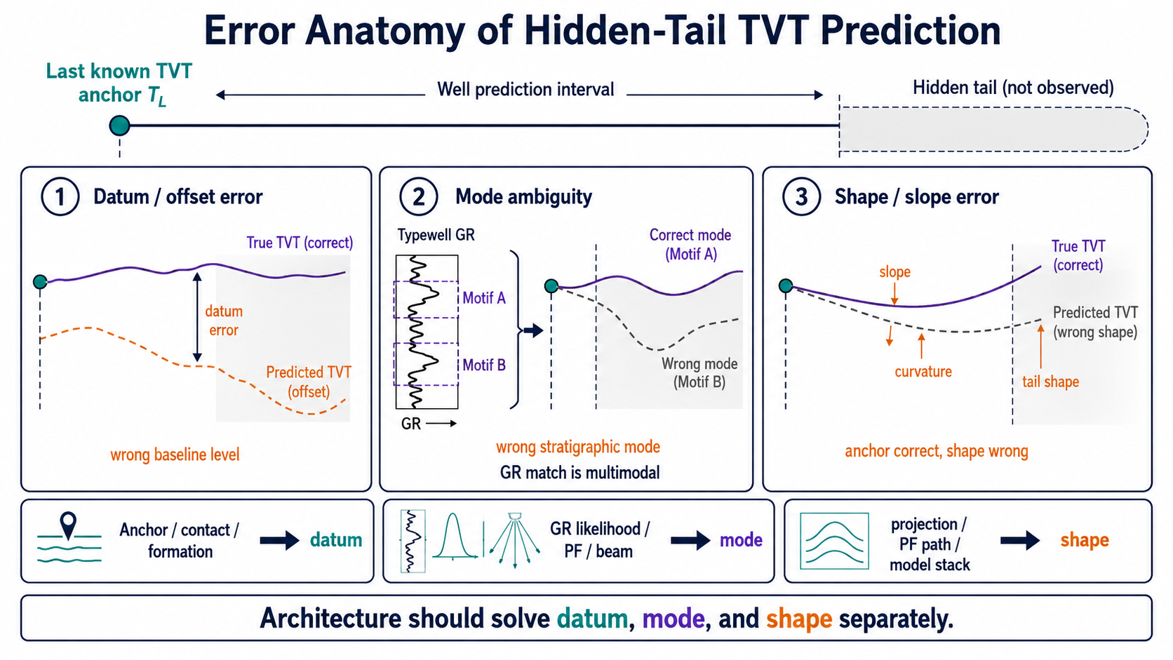
Suppose two candidate trajectories are $a_w(s)$ and $b_w(s)$, and branch $a$ is correct with probability $p$. The squared risk of hard selection is:

\[R_{hard}=(1-p)(a-b)^2.\]

The posterior mean $pa+(1-p)b$ has risk:

\[R_{mean}=p(1-p)(a-b)^2.\]

Therefore:

\[R_{hard}-R_{mean}=(1-p)^2(a-b)^2\ge0.\]

Without a reliable discriminator, hedging is more compatible with squared loss than a hard argmin. This motivated the bimodal detector, prefix-trust shrinkage, and visible-prefix guard. The final midpoint hedge reduced to:

if branch_mass >= 0.25 and 4.0 <= separation <= 40.0:
    midpoint = 0.5 * (low_branch + high_branch)
    shift = np.clip(0.60 * (midpoint - weighted_path), -2.0, 2.0)
    prediction[eval_mask] += shift

The branch had to be genuinely bimodal, both modes needed enough mass, and the resulting move was capped at 2 ft.

Because GR scale can differ between the typewell and horizontal well, I also fitted an affine heel calibration:

\[(\alpha_w,\beta_w) =\arg\min_{\alpha,\beta} \sum_{i\in\mathcal P_w} \left[G^{hw}_{w,i}-(\alpha G^{tw}_w(T^{input}_{w,i})+\beta)\right]^2,\] \[\widetilde G^{hw}_{w,i}=\frac{G^{hw}_{w,i}-\beta_w}{\alpha_w}.\]

Visible-prefix calibration, bimodal hedging, and guarded contact reconstruction brought public scores to roughly 7.2. The remaining problem was experimental attribution: when nearly identical functions moved by several hundredths on the leaderboard, one score did not identify the useful layer.

I changed the unit of experimentation from “one submission score” to “a preregistered hypothesis and a parent-child contrast.”

---

The 7.x cluster: when the public leaderboard became a shared search set

At this point, many competitors started from closely related public notebooks in the 7.x range. Their labels differed, but ridge alignment, particle filtering, projection, visible-prefix calibration, and contact reconstruction often produced predictions from the same family. Changing spread, projection degree, branch thresholds, or blend weights could move public score by a few hundredths. I ran many of those experiments as well.

In hindsight, two different kinds of value were being conflated.

• Structural value: public notebooks quickly exposed that the task was a trajectory problem involving datum, mode, and shape rather than ordinary row regression. That insight did contribute to private improvement.
• Selection value: finding the public-best cutoff or weight inside the same prediction family transferred very weakly. It selected a configuration that fit the visible evaluation slice, not necessarily one that generalized to unseen wells.

“Public notebooks were useful” and “continuing to tune their public parameters was useful” are therefore different claims. The first was largely true. The second became increasingly false once the field converged near 7.x.

Write the public measurement of candidate $\theta$ as:

\[\widehat R_{pub}(\theta) =R_{pub}(\theta)+\varepsilon_{sample}(\theta),\]

where $R_{pub}$ is risk under the public distribution and $\varepsilon_{sample}$ is finite-sample measurement error. The quantity we actually need is $R_{priv}$, but adaptive selection chooses:

\[\widehat\theta =\arg\min_{\theta\in\Theta_{adaptive}} \widehat R_{pub}(\theta).\]

This selects both genuinely good models and models whose public noise happened to be favorable. The final discrepancy has two distinct sources:

\[R_{priv}(\widehat\theta)-\widehat R_{pub}(\widehat\theta) = \underbrace{R_{priv}(\widehat\theta)-R_{pub}(\widehat\theta)}_{\text{distribution shift}} + \underbrace{R_{pub}(\widehat\theta)-\widehat R_{pub}(\widehat\theta)}_{\text{selection optimism}}.\]

Under the deliberately simple approximation of independent Gaussian measurement errors, the selection component grows roughly as:

\[\mathbb E\!\left[ \min_{1\le k\le K_{eff}}\varepsilon_{sample,k} \right] \approx -\sigma\sqrt{2\log K_{eff}}.\]

The candidates were highly correlated, so the effective number of trials $K_{eff}$ was smaller than the raw submission count. But $K_{eff}$ was also larger than any one person’s search. Once a favorable public configuration was shared, many competitors searched around it and published the next local optimum. The public leaderboard had become a community-wide adaptive search set, not an untouched validation set.

This competition also had a large gap between apparent sample size and effective sample size. The visible query contained 14,151 rows but only three wells. If row error is decomposed into a well-level datum error $\delta_w$ and local shape error $s_{w,i}$, then:

\[RMSE^2 =\sum_w\frac{n_w}{N} \left( \delta_w^2 +2\delta_w\overline{s}_w +\overline{s_w^2} \right).\]

A single datum mistake copies $\delta_w^2$ across the entire hidden tail of that well. Thousands of rows do not average this error away when they belong to only three correlated groups. A parameter that happens to fit one public well can move rank sharply, while one private well from another regime can reverse the ordering. The unusually large shake-up came from this combination: few independent groups, well-level error correlation, RMSE sensitivity to large misses, and community-wide adaptive search.

The final shake-up made this unusually visible. Herra Huu moved from public 1,591st (6.501) to private 15th (6.346), a gain of 1,576 positions and a gold medal. The absolute score improved by only 0.155. This was not 1,576 ranks’ worth of sudden private magic. It indicates that many teams ahead on public carried correlated errors, and the entire cluster was reordered when those errors met the private wells. In a dense score band, a modest absolute difference can expand into hundreds or thousands of ranks.

The right conclusion is neither “the public leaderboard was useless” nor “the climbers were merely lucky.” Public still identified large structural gains. Large risers may also have retained a different inductive bias, or selected a final submission that looked weaker on public but matched unseen wells better. What failed was the interpretation of public rank as a stable total ordering of model quality. It was partly a ranking within whichever model family the community had collectively optimized.

Observation	Tempting interpretation	Better interpretation and action
Many similar 7.x notebooks appear	The solution is nearly settled	One family has saturated the visible slice; search for a new observable
A weight change gains 0.02	Generalization improved	It may be adaptive optimism; test against a frozen parent and shift-aware holdout
A public low-rank team wins private gold	Hidden magic or luck explains everything	Correlated consensus error and rank compression were large; preserve orthogonal mechanisms
Public/private ordering changes sharply	Discard public evidence	Use it for large directional effects, not as a tie-breaker for small deltas

Public notebooks were therefore most useful when read like papers rather than answer keys. The transferable object was not the published weight. It was the new observable, the assumptions under which it worked, and a test capable of falsifying those assumptions. This is why the next phase decomposed notebooks into engines, observables, and artifacts before rebuilding them under common-parent OOF.

---

Phase 3: Decomposing public notebooks into source-complete experts

High-scoring public notebooks appeared quickly in July. The useful response was not to copy each notebook wholesale. I decomposed them with five questions:

1. What new observable does this notebook add?
2. Can it be reproduced without hidden targets?
3. Do train OOF and query inference use the same feature coordinate?
4. Is the parent prediction lineage identical across the comparison?
5. Are wells, rows, and columns discovered dynamically at runtime?

This separated public solutions into engines, observables, and artifacts. An executable query engine without common-parent OOF was not admitted as a strict expert. A good OOF model without a reproducible active-query feature builder was not deployable either.

The strict gate can be summarized as:

assert np.array_equal(parent_oof.id, feature_oof.id)
assert feature_manifest["target_columns_used"] is False
assert feature_manifest["coordinate_schema"] == query_schema

residual = y_true - parent_oof.prediction
model.fit(feature_oof.values, residual, groups=well_id)

query_feature = build_features(query, target=None)
assert query_feature.columns.tolist() == feature_oof.columns.tolist()

An attractive OOF number was not treated as deployable evidence unless this contract held.

The main families built during this phase were:

• query-aligned temporal residual routing;
• graph-distilled stratigraphic correction;
• station-local residual rows;
• TCN and HGBR graph experts;
• direct and residual BiMamba state-space experts;
• dip and formation structural fields;
• exact and content-verified trajectory transfer.

This opened the public 6.5 -> 6.0 range. It also rejected many models at strict fold gates. Rich features were not automatically better, mixed-lineage OOF produced large false gains, and a feature coordinate mismatch of only a few feet could invalidate a correction model.

Recording closed experiments mattered. Near the deadline, knowing which family had already failed was more valuable than generating another unconstrained idea.

---

Phase 4: Turning private-safe into an operational contract

Late in the competition, I developed a separate private-safe path. In hindsight, that term mixed two different claims.

Operational safety

• Hidden targets never enter the feature builder.
• ID and target columns are derived from sample_submission.csv.
• Well lists and row counts are never hard-coded.
• Frozen public-query features or predictions are not loaded.
• Dependencies are preserved in an owner-controlled private vault.
• Notebook and runtime artifact hashes are pinned.
• End-to-end inference passes within the Kaggle T4 nine-hour limit.

Statistical private generalization

• Corrections remain useful on unseen wells.
• The method does not depend excessively on visible-test exact/content overlap.
• OOF gains survive a shifted hidden distribution.
• A late layer does not worsen parent tail risk.

The first claim was achieved reasonably well. The final notebook derived the active schema, verified ID order and finite predictions, and dynamically processed all 14,151 visible query rows. I also built a dependency vault.

sample = pd.read_csv(comp_root / "sample_submission.csv", dtype=str)

id_matches = [
    c for c in sample.columns
    if str(c).strip().lower() == "id"
]
id_col = id_matches[0] if len(id_matches) == 1 else sample.columns[0]
target_cols = [c for c in sample.columns if c != id_col]

if len(target_cols) != 1:
    raise RuntimeError("could not derive the active target column")

parts = sample[id_col].str.rsplit("_", n=1, expand=True)
wells = parts.iloc[:, 0].astype(str)
rows = pd.to_numeric(parts.iloc[:, 1], errors="raise")

This contract eliminated the hidden-rerun format failures that had cost several submissions earlier.

The private result, however, shows that the second claim was not established strongly enough. A reproducible, leakage-controlled model is not automatically a distribution-robust model.

---

Architecture of the final notebook

The final notebook is internally titled Bounded Dual State-Space Structural Geosteering. It represents the selected PS3 branch and scored 5.998 public and 8.197 private.

The full path can be summarized as:

ridge/PF + physical selector
-> low-degree U = TVT + Z projection
-> learned trajectory blend
-> guarded contact / visible-prefix calibration
-> content-verified trajectory transfer
-> query-temporal risk-routed residual
-> graph-distilled correction
-> parent-specific datum head
-> dual BiMamba direct + residual correction
-> dip/formation structural field
-> dynamic schema and SHA audit

1. Ridge/PF and selector anchor

The first anchor combined two paths:

\[T_i^A=0.30T_i^{ridge}+0.70T_i^{selector}.\]

The selector used a 128-seed PF likelihood ensemble and a 14-configuration beam ensemble. PF scale and hold fraction changed with well length and $Z$ span.

2. Stratigraphic-level projection

The low-frequency projection was applied to:

\[U_i=T_i+Z_i.\]

The projected path was:

\[T_i^{proj} =(1-\lambda_p)T_i^A +\lambda_p\left(\widehat U_i-Z_i\right), \qquad \lambda_p=0.75.\]

This reduced row noise while preserving trajectory-scale shape. The notebook used an iteratively reweighted polynomial fit:

def robust_polyfit(s, y, degree=5):
    coef = np.polyfit(s, y, degree)
    for _ in range(4):
        residual = y - np.polyval(coef, s)
        scale = 1.4826 * np.median(np.abs(residual)) + 1e-6
        weight = 1.0 / (1.0 + (residual / (2.0 * scale))**2)
        coef = np.polyfit(s, y, degree, w=weight)
    return np.polyval(coef, s)

u_fit = anchor_u + robust_polyfit(s, (tvt + z) - anchor_u)
tvt_projected = 0.25 * tvt + 0.75 * (u_fit - z)

The repeated down-weighting kept isolated wrong-branch points from pulling the full curve.

3. Content-verified transfer

When query inputs identified an exact or partial labelled donor, the donor trajectory was calibrated to the prefix:

\[\widehat T_w^{content}(i) =T_d(MD_w(i)) +\operatorname{median}_{j\in\mathcal P_w} \left[T_w^{input}(j)-T_d(MD_w(j))\right].\]

All three visible query wells were identified as exact-copy cases by the content package. Identity alone was not enough: the donor still had to pass a visible-prefix check.

known = test_well[test_well["TVT_input"].notna()]
candidate = interpolate_donor(donor_tvt, known["MD"])
prefix_rmse = rmse(known["TVT_input"], candidate)

if len(known) >= 50 and valid_physics_rows >= 100 and prefix_rmse <= 1.0:
    prediction[hidden_rows] = interpolate_donor(donor_tvt, hidden_md)
else:
    prediction[hidden_rows] = parent_prediction[hidden_rows]

This was powerful on public and, for the same reason, statistically questionable on unseen private wells where the donor relationship might not exist.

4. Temporal risk router

Five parent paths and disagreement diagnostics were resampled to a 256-point coordinate. Fifteen temporal members predicted a degree-five Legendre correction:

\[r_w(s)=\operatorname{clip}\!\left[ 0.25\sum_{k=0}^{5}\theta_{w,k}P_k(2s-1),-8,8 \right].\]

A five-role risk ensemble used prediction-time summaries to estimate $\alpha_w\in[0,1]$:

\[\widehat T_w(s)=c_w(s)+\alpha_w r_w(s).\]

The residual was never added unconditionally. A target-free router converted disagreement and prefix-stability summaries into a bounded dose:

raw_residual = temporal_ensemble.predict(sequence_features)
router_input = summarize_without_target(parent_paths, raw_residual)
alpha = np.clip(risk_router.predict(router_input), 0.0, 1.0)

move = alpha[:, None] * np.clip(raw_residual, -8.0, 8.0)
prediction = content_parent + move

5. Graph, datum, BiMamba, and structural field

The late stack applied a source-complete graph TCN, parent-specific datum head, and dual BiMamba correction. The PS3 BiMamba layer contained 50 checkpoints, with direct dose 0.075 and residual dose 0.5.

The final structural field dynamically combined dip and formation predictions as a small bounded correction:

\[\Delta^{struct}_w =0.5\left[ 0.1\,\operatorname{clip}(\Delta^{dip}_w,-4,4) +0.075\,\operatorname{clip}(\Delta^{formation}_w,-4,4) \right].\]

Every layer was recomputed from the active query. The final audit derived the live schema from sample_submission.csv rather than assuming a row count or target name:

sample = pd.read_csv(sample_path)
submission = pd.read_csv(submission_path)

identifier = sample.columns[0]
prediction_col = [c for c in sample.columns if c != identifier][0]

if submission.columns.tolist() != sample.columns.tolist():
    raise RuntimeError("submission columns differ from sample")
if not submission[identifier].astype(str).equals(sample[identifier].astype(str)):
    raise RuntimeError("identifier order differs from sample")

values = submission[prediction_col].to_numpy(float)
if not np.isfinite(values).all():
    raise RuntimeError("submission contains non-finite predictions")

audit["sha256_submission_csv"] = sha256_file(submission_path)

This operational contract is the most reusable part of the final notebook.

---

The final 3+2 portfolio

On the last day, I avoided repeating already scored functions and prepared three mechanism-diverse moonshots plus two private-safe candidates.

Role	Candidate	Public	Private	Gap
Moonshot	M4 residual direct structural	6.103	8.202	+2.099
Moonshot	M5 TCN dual structural	6.066	8.034	+1.968
Moonshot	M3 HGBR direct structural	6.060	8.132	+2.072
Private-safe	PS1 bounded residual structural	5.952	8.523	+2.571
Private-safe	PS3 bounded TCN dual structural	5.998	8.197	+2.199

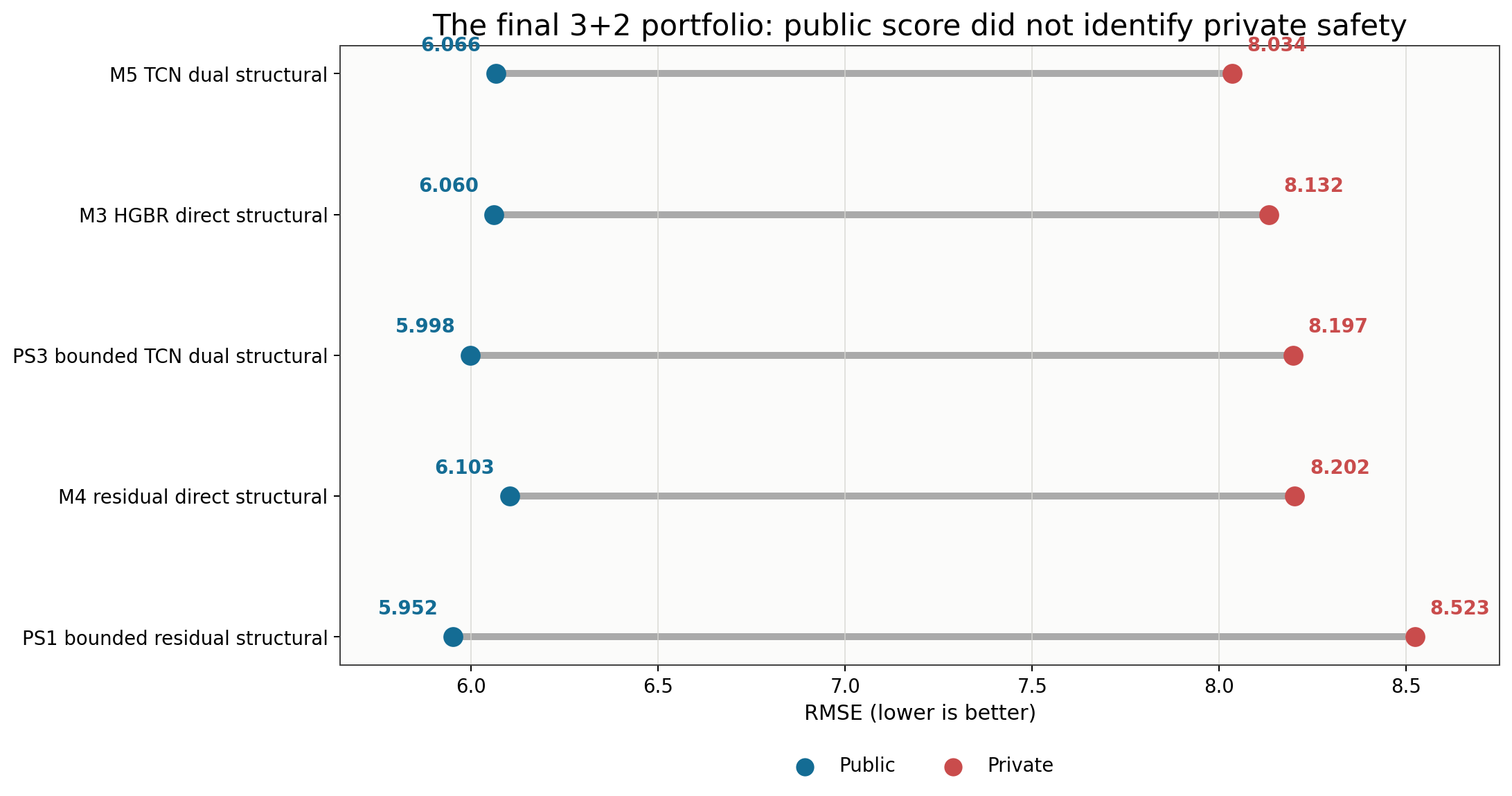
Public ordering was PS1 -> PS3 -> M3 -> M5 -> M4. Private ordering was M5 -> M3 -> PS3 -> M4 -> PS1. The public-best PS1 was the private-worst of the five.

The official team private score 8.197 exactly matches PS3, so PS3 determined the final result among the two selected submissions. With hindsight, M5’s 8.034 was my best private score across the entire ledger. Selecting it would have implied roughly rank 170 under the same final ordering, around 40 positions above the actual 210th. That would have helped, but it would not have changed the central conclusion.

The naming is the more important lesson. PS1 and PS3 were called private-safe because they had dynamic schema handling, bounded corrections, owner-controlled dependencies, and a no-target contract. The name did not establish statistical superiority under the private distribution. Future work should separate the terms explicitly:

deployment-safe: reproducible, leakage-controlled, schema-safe
distribution-robust: validated under a credible unseen-group shift

---

Lessons worth carrying forward

1. Changing the problem representation

Moving from row regression to datum/mode/shape decomposition produced the largest useful improvement. Private score improved from 13.743 to 8.197, not just public score.

2. Treating prefix and typewell as evidence rather than commands

Prefix calibration, heel GR calibration, and contact reconstruction were strong. Converting them from unconditional overrides into guarded evidence reduced catastrophic failures.

3. Enforcing source-complete dynamic inference

Late in the competition, model OOF was secondary to four questions:

Can the exact feature be rebuilt on a new well?
Does the same parent exist in OOF and query inference?
Does target mutation leave the prediction unchanged?
Can the notebook derive all IDs and columns at runtime?

This discipline allowed the final notebooks to complete without format failures.

4. Moving experiments into a file-backed ledger

Each hypothesis had an expected outcome, actual score, implication, and next action stored in CSV, JSON, or Markdown. Near the deadline, this ledger was more valuable than memory. It prevented retraining closed families and allowed result-conditioned branches to be prepared before scores arrived.

5. Reading public notebooks as candidates for independent experts

I did not simply append public code. I isolated observables and model families and rebuilt them under strict OOF. Many branches failed, but temporal residuals, graph TCN, and BiMamba produced genuine private improvement.

---

What I would improve

1. Public score remained the primary objective for too long

Across 301 identical-submission pairs, public/private Spearman correlation was 0.763. Directional information existed, but it was insufficient for final selection. 90.0% of my paired submissions became worse on private, with a median gap of +2.310.

Public PB hunting was useful for feature discovery. Late in the competition, however, transfer estimation should have replaced it as the primary objective.

2. Visible-query overlap was overvalued as a generalization signal

The visible sample contained three wells and 14,151 rows. Exact and content-verified transfer was very strong on that coordinate. The same donor relationship need not exist for unseen private wells.

A rule perfectly verified on visible query inputs can still be a conditional shortcut rather than a robust model.

3. OOF did not simulate the hidden distribution well enough

Grouped well folds prevented row leakage, but they did not reproduce the private shift. A stronger pseudo-private split could have held out wells with:

• distant typewell families;
• unstable prefix GR calibration;
• bimodal likelihood landscapes;
• long hidden tails and large $Z$ span;
• no donor or content match.

Only validation under this kind of shift would justify a statistical private-safe claim.

4. More layers were mistaken for more independent information

The final notebook contains many models, but several read different transforms of the same parent disagreement. Increasing model count does not increase information when the sources are correlated.

M5’s better private result relative to PS1 suggests that mechanism diversity and bounded transfer mattered more than the last few hundredths of public RMSE.

5. Final selection needed a more direct correction-risk objective

I considered public score, OOF gain, source diversity, and runtime safety. The private reveal suggests a stronger objective:

\[J_{final} =\widehat{RMSE}_{shift} +\lambda_1\,Q_{0.95}(|\Delta|) +\lambda_2\left|\operatorname{Corr}(\Delta,\Delta_{parent})\right| +\lambda_3 D_{overlap}.\]

Here $D_{overlap}$ measures dependence on exact or content overlap in the visible query. Average OOF gain should be penalized by correction tails, redundancy with the parent, and query-specific dependence.

---

How to read the public/private gap

It is also too strong to conclude that the public leaderboard was useless. While public improved from 14.288 to 5.952, private improved from 13.743 into the low 8s. Large structural gains transferred.

The weak transfer appeared mainly in late, small, and query-specific gains:

large structural gain
  -> often transfers

query-specific alignment or overlap gain
  -> may transfer weakly or not at all

small late-stage blend gain
  -> difficult to distinguish from evaluator noise and shift

The leaderboard should therefore be treated as a noisy measurement, not the objective itself.

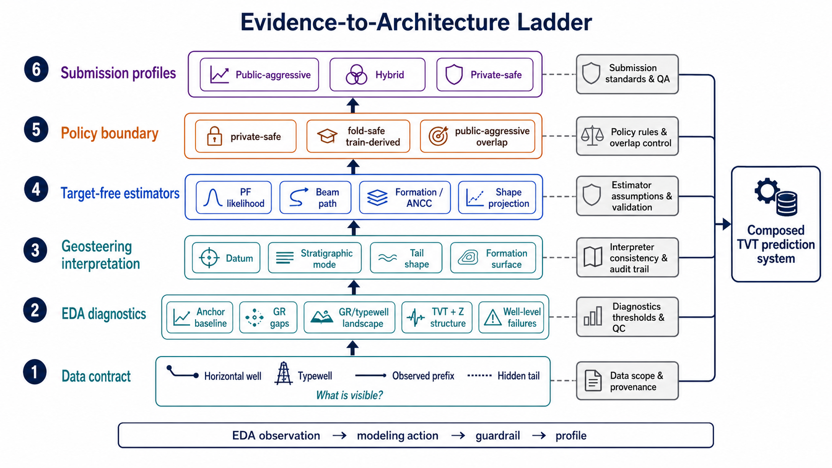
A better sequence is:

\[\text{observation} \rightarrow \text{estimator} \rightarrow \text{shift-aware validation} \rightarrow \text{bounded deployment policy} \rightarrow \text{leaderboard confirmation}.\]

This competition exposed the remaining gap between the last two steps.

---

How I would approach the competition again

First week

1. Automate sample-schema and hidden-rerun contracts immediately.
2. Build a shift-aware holdout in addition to grouped-well OOF.
3. Compute datum/mode/shape decomposition and oracle ladders first.
4. Treat public notebooks as an observable inventory rather than a score inventory.

Middle phase

1. Freeze the parent and evaluate only one correction at a time.
2. Hash every correction vector and OOF row identity.
3. Track average gain, well-win rate, and p95/p99 damage together.
4. Spend GPU time only on source-complete models that pass fold 0.

Final two weeks

1. Maintain separate boards for public-aggressive and distribution-robust candidates.
2. Repeat identical functions only enough to estimate measurement noise.
3. Spend submissions on main-effect and interaction contrasts.
4. Choose the final two by mechanism diversity and shift risk, not public ordering.

I would also change the final portfolio objective to:

\[\min_{a,b} \mathbb E_{\mathcal D_{shift}} \left[\min\{L(a),L(b)\}\right] +\lambda\,\operatorname{Corr}(e_a,e_b),\]

where the two candidates need both low expected loss and distinct failure modes.

---

Closing

The final result was 210th place and a silver medal. It was below what a public score of 5.952 appeared to promise, and the private score of 8.197 makes the lack of late-stage transfer unambiguous.

I still do not read the project as a simple failure.

• Private improved from 13.743 to 8.197.
• The task was reframed as target-free geosteering.
• Error was separated into datum, mode, and shape.
• The boundary between hidden targets and observed covariates became a code contract.
• Source-complete OOF was connected to dynamic inference.
• The final notebook deployed 50 state-space checkpoints and a structural field through one reproducible path.
• Most importantly, the difference between public score and private robustness became measurable rather than rhetorical.

The final notebook is not a minimal solution. It is closer to a research record of how far several months of ideas could be composed into one system. The most reusable output is not the stack itself, but the operating principle it left behind:

Recover datum when evidence is strong.
Hedge mode when evidence is ambiguous.
Model shape only in a consistent coordinate.
Treat reproducibility and generalization as separate claims.
Use the leaderboard as evidence, never as the definition of truth.

The silver medal was the result. The public/private gap was the final lesson.

---

References

• ROGII - Wellbore Geology Prediction
• ROGII final leaderboard
• Pilkwang Kim, ROGII Development & Tests
• Pilkwang Kim, Working Note: Target-Free TVT Geosteering
• Georgy Mamarin, Stop reforking: the best GR fit is the wrong depth
• ROGII Geological Operations / StarSteer overview
• mycarta, ROGII Geosteering Toolkit

Leaderboard analysis note

Statistics were computed on August 6, 2026 from the official Kaggle API: 6,191 matched public/private team rows and my personal submission ledger. Team-level scores may come from different selected submissions and are used for standings shake-up analysis. Personal submission gaps pair the same submission reference directly.