PG S6E6: Redshift, Color Geometry, and OOF Artifact Blending

PG S6E6: Redshift, Color Geometry, and OOF Artifact Blending

Competition link:
Playground Series S6E6

Kaggle code:
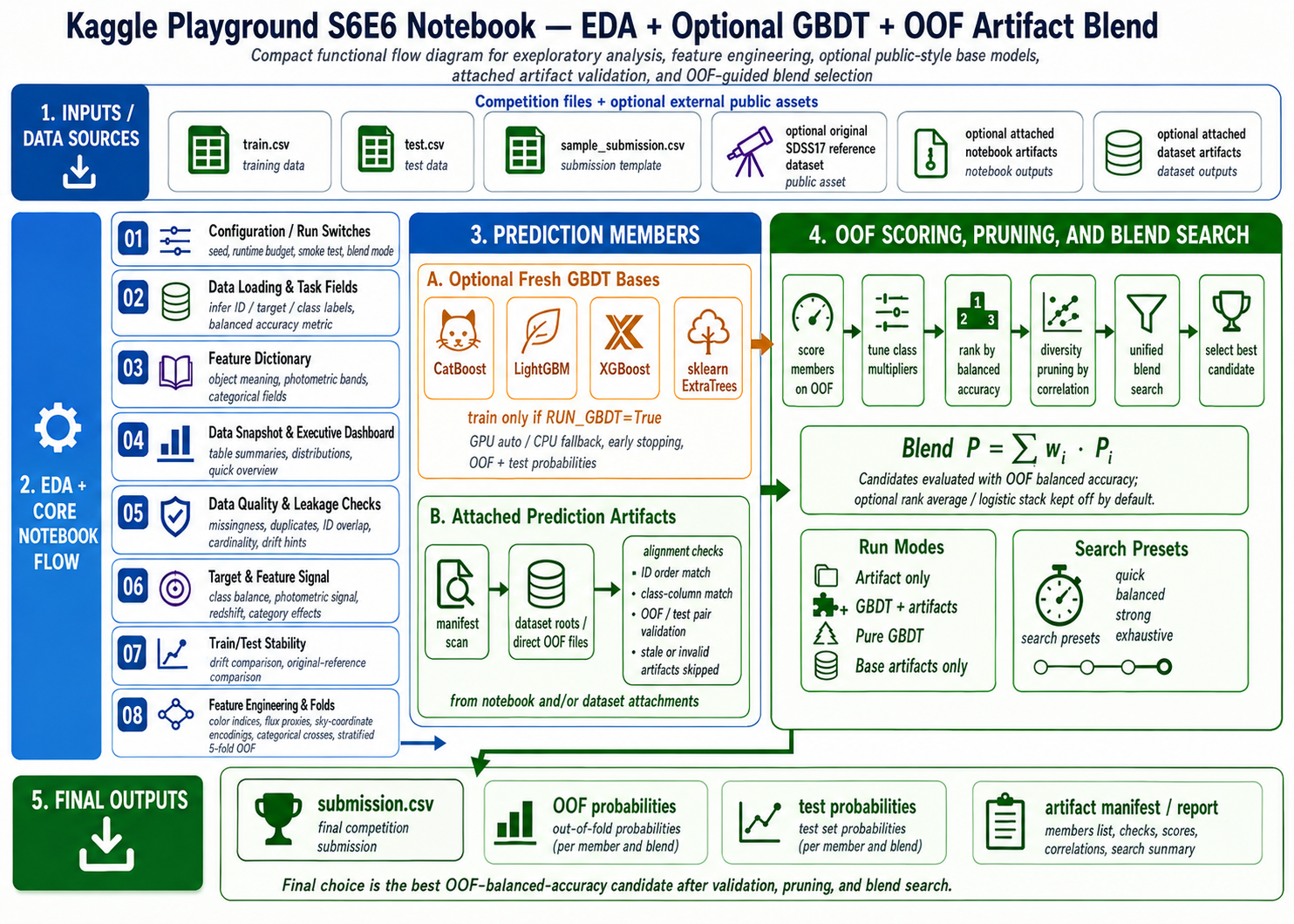
PG S6E6 EDA + GBDT Bases + Artifact Blend

The modeling object is a metric-aware probability system for stellar-class labels.

The task is a three-class hard-label classification problem:

GALAXY / QSO / STAR

The scoring metric is balanced accuracy, so the central question is not:

Which model gets the most rows correct?

It is:

Which model preserves recall across all three astrophysical classes?

That distinction determines the EDA, the feature engineering, the fold design, the artifact intake rules, the blend search, and the final class multipliers.

Dependency order: metric first, feature meaning second, OOF evidence third, and blend calibration last.

The selected blend reaches:

Quantity	Value
Best single OOF BA	0.968129
Selected blend OOF BA	0.969191
OOF BA gain	+0.001062
OOF log loss	0.091453
OOF macro-F1	0.952234

The OOF gain is a small residual correction on top of a strong artifact member.

1. The Metric Comes First

The train distribution is imbalanced:

Class	Share
GALAXY	0.653818
QSO	0.202899
STAR	0.143283

Under ordinary accuracy, a model can lean toward GALAXY and still look strong. Under balanced accuracy, each class receives equal metric weight:

\[\operatorname{BA} = \frac{1}{K} \sum_{k=1}^{K} \frac{\operatorname{TP}_k}{\operatorname{TP}_k + \operatorname{FN}_k}\]

For this competition, K = 3. The score is therefore an average of recall for GALAXY, QSO, and STAR.

This changes the optimization target from row-level correctness to class-wise coverage. Class-weighted training and OOF class-multiplier search follow directly from this objective.

The corresponding inverse-prior style weights are:

Class	Train Share	Weight
GALAXY	0.653818	0.509826
QSO	0.202899	1.642856
STAR	0.143283	2.326397

The meaning is straightforward: being wrong on STAR is not numerically rare noise. It is one third of the official metric.

2. What The Dataset Is Really Saying

The raw input table is compact:

Feature Family	Columns
sky position	alpha, delta
photometric magnitudes	u, g, r, i, z
redshift	redshift
categorical context	spectral_type, galaxy_population

The statistical reading does not treat all columns as generic tabular fields. Each column is interpreted by the physical information it carries.

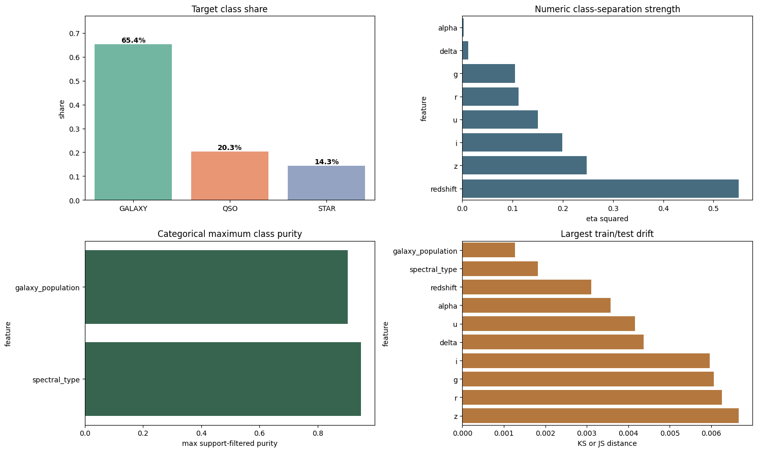
The first signal is that redshift dominates the raw numeric screen. The effect-size screen reports:

Feature	eta squared
redshift	0.55006
z	0.24737
i	0.19920
u	0.15091
r	0.11217
g	0.10464

The statistic here is an effect-size view. One way to read eta squared is:

\[\eta^2 = \frac{\text{between-class variation}} {\text{total variation}}\]

So redshift is not merely correlated with the target. It explains a large share of class-separating variation.

The second signal is categorical purity. The strongest categorical field, spectral_type, reaches a maximum support-filtered class purity of about 0.94956. galaxy_population reaches about 0.90285.

These values do not mean the categorical variables solve the problem. They mean the tree models should be allowed to exploit categorical splits, and the feature engineering should preserve interactions between categorical context and photometric/redshift behavior.

3. Redshift Is A Separator, Not A Complete Rule

The redshift distribution explains why the problem is easy in some regions and ambiguous in others.

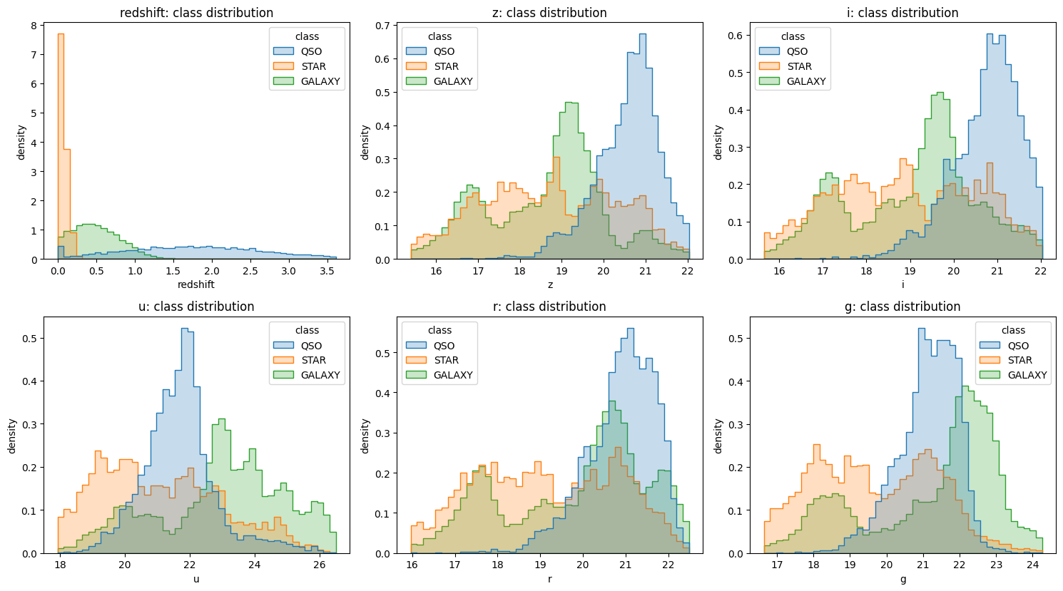
The class medians tell the story:

Class	Redshift Median
STAR	0.05649
GALAXY	0.48196
QSO	1.79889

The intuition is:

STAR   -> near-zero redshift
GALAXY -> moderate redshift
QSO    -> often high redshift

But this is not a hard rule. There is overlap near low redshift and in the broad magnitude distributions. That overlap is where a probability model matters.

If one made a crude rule such as:

\[\hat{y} = \begin{cases} \text{STAR}, & z_{\text{redshift}} < \tau_1 \\ \text{QSO}, & z_{\text{redshift}} > \tau_2 \\ \text{GALAXY}, & \text{otherwise} \end{cases}\]

it would capture part of the physical structure but fail in mixed regions. A richer representation uses redshift as one axis inside a broader feature space.

4. Why Magnitude Becomes Color

The five band columns u, g, r, i, z are magnitudes. Magnitudes are logarithmic measurements, so differences between magnitudes are more physically meaningful than many raw comparisons.

The key transformation is a color index:

\[\operatorname{color}_{a,b} = m_a - m_b\]

Because astronomical magnitude relates to flux by:

\[m \propto -2.5\log_{10}(F)\]

a magnitude difference is equivalent to a flux ratio:

\[\frac{F_a}{F_b} = 10^{-0.4(m_a - m_b)}\]

The feature set therefore contains both:

u_minus_g, g_minus_r, r_minus_i, i_minus_z, ...
flux_ratio_u_g, flux_ratio_g_r, ...

This is not decorative feature expansion. It is a way to turn raw band brightness into spectral shape.

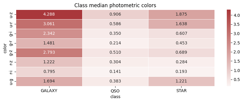
The median color heatmap makes this clear:

For example:

Color	GALAXY	QSO	STAR
u-z	4.288	0.906	1.875
u-r	3.061	0.586	1.638
g-i	2.342	0.350	0.607
g-r	1.481	0.214	0.453

The GALAXY median is much redder in these broad colors. QSO is comparatively flatter across these bands. STAR sits in between for some colors and overlaps heavily elsewhere.

This motivates a feature family rather than a single feature:

Feature Family	Why It Exists
color differences	capture spectral slope and class separation
flux ratios	express the same color relation in a multiplicative scale
magnitude summaries	summarize overall brightness and shape
redshift interactions	let color behavior depend on redshift

The scatter of redshift and u-z shows why this interaction matters:

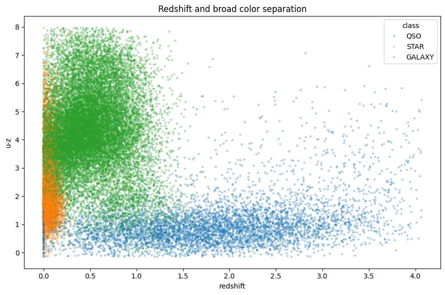
There are visible class regions, but they are not linearly separable everywhere. This is the ideal setting for GBDT models: many meaningful axes, nonlinear thresholds, and local interactions.

Snippet: color and flux-ratio features

color_pairs = [
    ("u", "g"), ("g", "r"), ("r", "i"), ("i", "z"),
    ("u", "r"), ("u", "i"), ("u", "z"),
    ("g", "i"), ("g", "z"), ("r", "z"),
]

for a, b in color_pairs:
    color = out[a] - out[b]
    out[f"{a}_minus_{b}"] = color
    out[f"{a}_div_{b}"] = safe_divide(out[a], out[b])
    out[f"flux_ratio_{a}_{b}"] = np.power(
        10.0, -0.4 * color.clip(-50, 50)
    ).astype("float32")

5. Why Redshift Is Expanded

redshift has the strongest raw effect size, but a single real-valued feature can still be awkward for tree models and neural artifacts. It is expanded into several forms:

Feature	Role
redshift_abs	handle negative or near-zero behavior symmetrically
redshift_sq	amplify high-redshift regimes
redshift_log1p	compress long right tail
redshift_signed_log1p	preserve sign while compressing scale
near_zero_redshift	mark likely stellar or local objects
high_redshift	mark quasar-like regimes
very_high_redshift	isolate extreme QSO-like cases

Conceptually, this is a basis expansion:

\[x \rightarrow \phi(x) = \left[ x,\ |x|,\ x^2,\ \log(1+x_+),\ \mathbf{1}(|x|<0.1),\ \mathbf{1}(x>1),\ \mathbf{1}(x>2) \right]\]

This lets different model families use the same physical feature in different ways. A tree can split on high_redshift. A neural artifact can use the smooth transformed value. A blend can benefit from both.

The feature space also includes interactions such as:

\[\text{redshift} \times (u-z)\]

The modeling meaning is:

A color difference may imply different classes depending on where the object sits in redshift space.

That is the right interpretation for a mixed stellar/galaxy/quasar classification task.

6. Astronomy-Oriented EDA Geometry

Astronomy-oriented EDA geometry sits closer to the measurement process than a plain feature-importance table. The useful signals are not just “which column is strong”; they are where the class boundary bends and which feature families should be trusted as priors rather than labels.

Categorical association can be summarized with Cramer’s V:

\[V = \sqrt{ \frac{\chi^2} {n\cdot \min(r-1,\ c-1)} }\]

where r and c are the contingency-table dimensions. The two categorical fields are not decorative:

Feature	Cramer’s V With Class	Modeling Meaning
galaxy_population	0.59349	strong population prior
spectral_type	0.52480	strong spectral prior

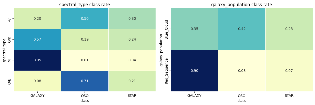
The heatmap explains why categorical variables are preserved and crossed with redshift flags. M is almost entirely GALAXY; O/B leans heavily toward QSO; Red_Sequence is mostly GALAXY. But Blue_Cloud remains mixed, and several spectral groups still contain nontrivial minority classes. So these fields should act as high-quality priors, not deterministic replacement labels.

The color-color plane then shows why the magnitude features are expanded into multiple color differences instead of reduced to one brightness score.

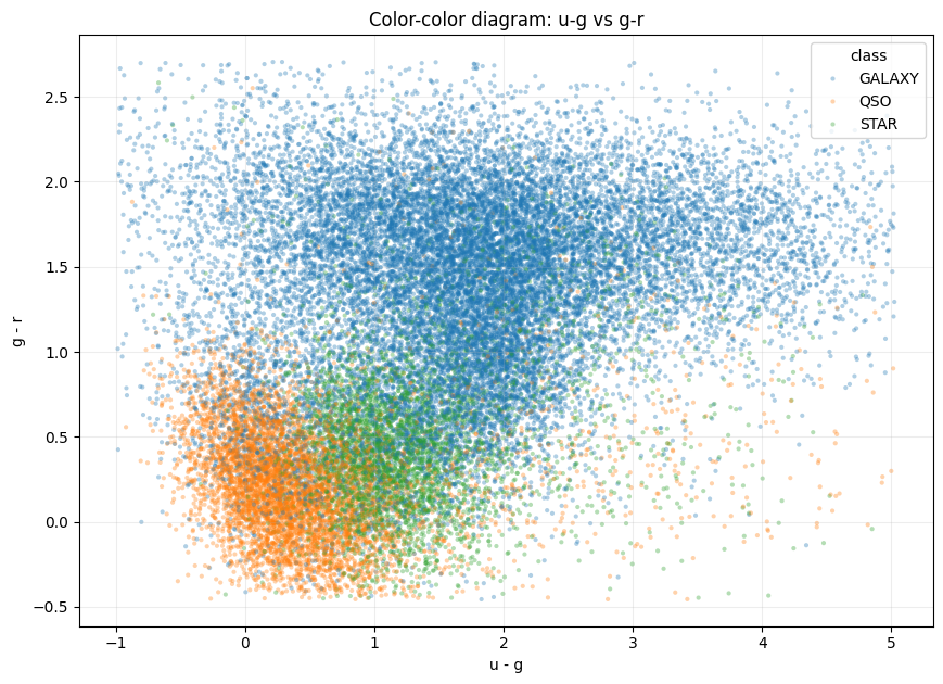
The two axes:

\[\Delta_{ug}=u-g, \qquad \Delta_{gr}=g-r\]

approximate adjacent spectral slopes. QSO occupies a lower g-r band, GALAXY forms a large higher g-r cloud, and STAR overlaps both in the middle. That overlap is important: color geometry creates strong regions, but not an axis-aligned rule. GBDT splits and neural probability artifacts are therefore useful because they can represent curved and locally mixed decision surfaces.

The redshift ECDF makes the threshold logic more explicit:

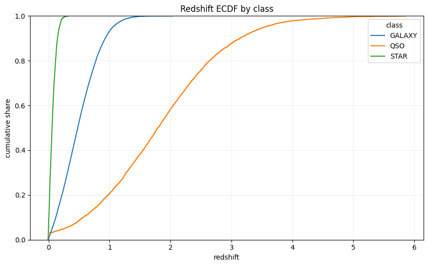
For class c, the curve is:

\[F_c(z) = P(\text{redshift}\le z\mid y=c)\]

STAR accumulates near zero redshift, GALAXY occupies the intermediate regime, and QSO keeps a long high-redshift tail. This supports the explicit flags near_zero_redshift, high_redshift, and very_high_redshift. Those flags are not arbitrary bins; they mark different parts of the class-conditional cumulative distribution.

The dataset-level ECDF view separates competition drift from original-reference drift:

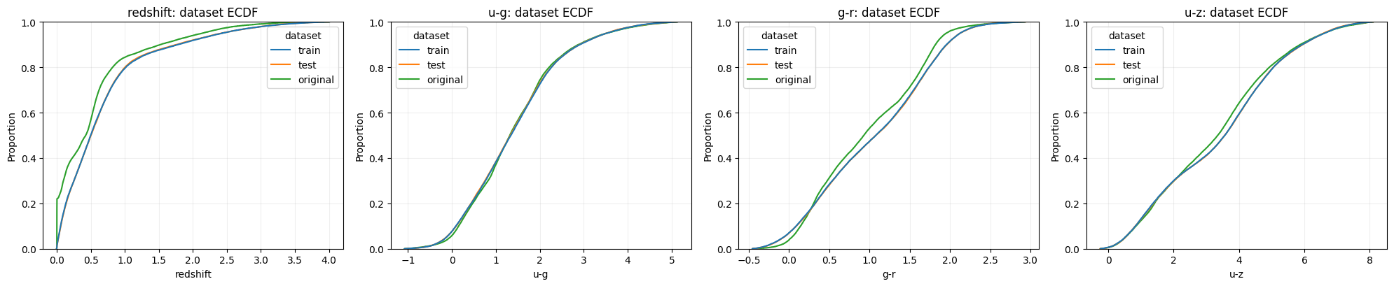
Train and test nearly overlap for redshift, u-g, g-r, and u-z. The original reference table is visibly different, especially in redshift and some photometric tails. The raw diagnostic table also shows -9999 sentinel values in original u, g, and z, while competition train/test have no such sentinel counts. That makes the original data useful for physical intuition, but risky as an unweighted validation proxy.

Finally, alpha and delta should be treated as sky geometry rather than ordinary independent numeric columns.

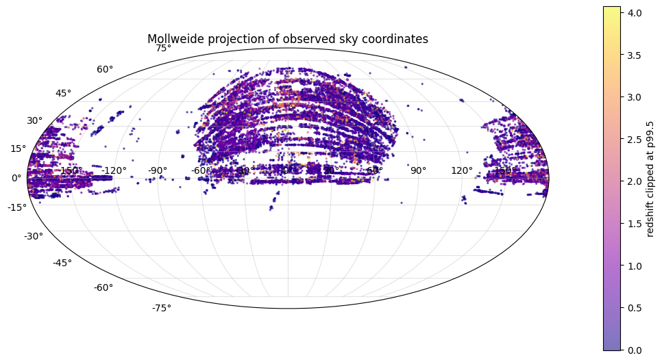
The projection shows a survey footprint, not a uniformly sampled sphere. Coordinate position may encode selection effects, but right ascension also wraps at 0 degrees / 360 degrees. Periodic and spherical encodings are safer than raw-angle-only splits:

Snippet: sky geometry and categorical crosses

alpha_rad = np.deg2rad(out["alpha"])
delta_rad = np.deg2rad(out["delta"])

out["alpha_sin"] = np.sin(alpha_rad).astype("float32")
out["alpha_cos"] = np.cos(alpha_rad).astype("float32")
out["delta_sin"] = np.sin(delta_rad).astype("float32")
out["delta_cos"] = np.cos(delta_rad).astype("float32")

out["sky_x"] = out["delta_cos"] * out["alpha_cos"]
out["sky_y"] = out["delta_cos"] * out["alpha_sin"]
out["sky_z"] = out["delta_sin"]

out["spectral_population"] = (
    out["spectral_type"].astype(str)
    + "__"
    + out["galaxy_population"].astype(str)
)
out["spectral_highz"] = (
    out["spectral_type"].astype(str)
    + "__highz_"
    + out["high_redshift"].astype(str)
)

The full modeling consequence is:

EDA Geometry	Feature Consequence
categorical class-rate heatmaps	keep categorical features and use categorical crosses
color-color overlap	use many color differences and flux-ratio transforms
class-wise redshift ECDF	add redshift basis expansion and threshold flags
train/test ECDF alignment	trust competition OOF more than original-reference validation
sky-coordinate footprint	encode angles periodically and add spherical coordinates

7. Drift Checks Are About Trust

The geometry plots give the visual version of the trust question. The drift statistics quantify it: how close are the distributions that generate OOF rows and test rows?

The largest raw train/test drift is small:

Feature	Drift Statistic
z	0.00666
r	0.00626
g	0.00606
i	0.00596
redshift	0.00311

For numeric features, KS-style distribution distance measures the largest gap between empirical distributions:

\[D_{KS} = \sup_x \left| F_{\text{train}}(x) - F_{\text{test}}(x) \right|\]

For categorical features it uses Jensen-Shannon distance.

The conclusion is not “there is no distribution shift.” The conclusion is narrower:

The public train/test split does not show large univariate raw-feature drift.

That supports using competition-fold OOF estimates and attached artifacts, as long as those artifacts are aligned to the same competition rows.

The original SDSS17 reference is different. It has a different class prior and a much larger redshift distribution shift against the competition train table:

Comparison	Signal
original STAR share minus competition train STAR share	+0.07266
original vs competition redshift KS	0.19553

This is why the original reference is useful for feature intuition but dangerous as an unexamined training distribution. It can inform the astrophysical reading; it should not silently define the validation target.

8. OOF As Evidence

Probability sources are not interchangeable until they earn trust through OOF behavior:

Every probability source must first behave well on rows it did not train on.

For row i, OOF prediction means:

\[\hat{p}^{\text{OOF}}_i = f_{-k_i}(x_i)\]

where k_i is the validation fold containing row i, and f_{-k_i} is trained without that fold.

This matters because in-sample predictions answer the wrong question. They ask:

How well can the model describe rows it already saw?

OOF predictions ask:

How well does this modeling recipe behave on unseen rows drawn from the same training distribution?

OOF serves four roles:

OOF Role	Meaning
score fresh GBDT bases	estimate each model’s metric contribution without training-row leakage
validate attached artifacts	accept external probability files only if their OOF side is row/class aligned
prune correlation	compare members by OOF probability geometry
search blend weights	choose weights using the same metric the competition rewards

This is why artifact loading is not merely a file-management step. An artifact is not trusted because it has a good name or a good public score. It is trusted only if it provides a compatible OOF probability matrix and a matching test probability matrix.

9. Fresh GBDT Bases As Local Anchors

CatBoost, LightGBM, and XGBoost are trained on the engineered feature frame. Their OOF scores are strong:

Model	OOF BA	OOF Log Loss
public_xgboost	0.965352	0.098110
public_catboost	0.964304	0.112588
public_lightgbm	0.964266	0.095724

These models are not the final center of gravity, but they have a specific purpose:

1. They verify that the engineered features are genuinely predictive.
2. They provide fresh, reproducible OOF/test probability members.
3. They add tree-shaped decision surfaces to a pool dominated by attached artifacts.

The strong neural artifact is better than the fresh GBDTs, but the GBDTs still matter because they make different local mistakes. That is why the final blend gives them nonzero weight.

Snippet: fold-safe GBDT probability generation

for fold in range(N_FOLDS):
    trn_idx = np.where(fold_id != fold)[0]
    val_idx = np.where(fold_id == fold)[0]

    model.fit(X_train.iloc[trn_idx], y[trn_idx])

    oof[val_idx] = normalize_probs(
        model.predict_proba(X_train.iloc[val_idx])
    )
    test_probs += normalize_probs(
        model.predict_proba(X_test)
    ) / N_FOLDS

The averaged test prediction is:

\[\hat{p}^{\text{test}} = \frac{1}{K} \sum_{k=1}^{K} f_{-k}(x_{\text{test}})\]

That keeps the validation and test prediction recipes aligned.

10. Artifact Blending Is A Second-Order Model

The strongest single member is:

Member	Source	OOF BA
realmlp_pytorch_5fold_6epoch	attached artifact	0.968129

The selected blend is not trying to replace it. It is trying to correct it.

Let p_m(x) be the probability vector from member m. A probability blend is:

\[p_{\text{blend}}(x) = \sum_{m=1}^{M} w_m p_m(x), \qquad w_m \ge 0,\quad \sum_m w_m = 1\]

The final selected weights show the intended behavior:

Member	Weight
realmlp_pytorch_5fold_6epoch	0.62239
public_lightgbm	0.18710
realmlp_seed2026_full_fullrows_fullorig_5fold	0.05725
public_catboost	0.05381
high-score stack artifact	0.03036
RealMLP full artifact	0.02729
public_xgboost	0.02071
Cat artifact	0.00110

This is not democratic averaging. It is a dominant-member blend. The best artifact keeps most of the mass; GBDT and other artifacts become structured residual corrections.

That is the reason the gain is small but plausible. A model pool with already strong members rarely gains by averaging everything. It gains by finding the few places where another model’s probability geometry improves class recall.

11. Correlation Pruning Prevents Fake Diversity

Many artifacts have impressive scores but extremely high OOF correlation. That is expected: many tabular pipelines learn similar class boundaries from the same redshift/color/categorical signal.

The pruning logic asks:

\[\rho_{ij} = \operatorname{corr} \left( \operatorname{vec}(P_i^{OOF}), \operatorname{vec}(P_j^{OOF}) \right)\]

If a lower-scoring member has near-duplicate OOF probabilities against an already-kept member, it contributes little except extra blend search noise.

Examples from the kept pool:

Pair	OOF Corr	Disagreement
RealMLP PyTorch vs public XGBoost	0.990921	0.018535
RealMLP PyTorch vs public CatBoost	0.988360	0.022361
RealMLP PyTorch vs public LightGBM	0.989980	0.019027
RealMLP PyTorch vs high-score stack	0.985997	0.023951

Even kept models are highly correlated. That tells us the blend should be conservative.

The resulting rule is:

Diversity is not model-name diversity. Diversity is OOF error-geometry diversity.

12. Class Multipliers Are Metric Calibration

The selected blend’s raw probabilities are not the final hard labels. For balanced accuracy, the decision boundary can be adjusted by class multipliers:

\[\hat{y} = \arg\max_c \left[ \lambda_c p_c(x) \right]\]

The selected multipliers are:

Class	Multiplier
GALAXY	0.770524
QSO	1.020000
STAR	1.275000

This is an explicit correction for the metric. GALAXY is the majority class, so its probability is discounted. STAR is the smallest class, so it is promoted.

That does not mean the model is pretending STAR is more common. It means the final decision rule is tuned for equal class recall rather than maximum raw accuracy.

This is the difference between probability estimation and metric-optimal classification:

\[p(y=c \mid x) \quad \text{estimates class probability}\]

but:

\[\arg\max_c \lambda_c p(y=c \mid x) \quad \text{chooses the label under the target metric}\]

The final submission class share reflects this:

Class	Train Share	Submission Share
GALAXY	0.653818	0.632223
QSO	0.202899	0.208047
STAR	0.143283	0.159731

The shift is not arbitrary. It is a consequence of optimizing recall balance.

13. Artifact Output As A Probability Object

A reusable artifact represents:

OOF probabilities + test probabilities + manifest + selected blend metadata

That bundle turns the final probability system into a future blend member. The artifact loop is recursive:

1. It consumes prior artifacts.
2. It evaluates them through OOF.
3. It blends them with fresh GBDT bases.
4. It emits a new validated probability artifact.

The selected output is:

Artifact	Kind	OOF BA	OOF Log Loss	OOF Macro-F1
eda03_gbdt_artifact_blend	selected:dirichlet_blend_22	0.969191	0.091453	0.952234

This is why artifact hygiene matters. If each run emits row-safe OOF/test probabilities, future blends can compose them without rerunning every model. If a run emits only a submission file, most of the statistical information is lost.

14. Modeling Consequences

The modeling dependency chain is:

metric -> feature meaning -> OOF evidence -> probability geometry -> calibrated decision rule

The feature evidence explains why the transformations exist:

Observation	Modeling Consequence
redshift has dominant class effect size	expand redshift and interact it with colors
magnitudes are logarithmic	use color differences and flux ratios
color-color and redshift ECDF geometry are class-conditional	use nonlinear local learners rather than one-threshold rules
sky coordinates have survey-footprint structure	encode angular geometry instead of only raw degrees
categorical purity is high	preserve categorical splits and crosses
train/test raw drift is small	trust fold-based competition OOF more than original-reference assumptions
class prior is imbalanced	optimize balanced accuracy, not ordinary accuracy

The OOF evidence explains why the blend is credible:

OOF Evidence	Modeling Consequence
RealMLP artifact is strongest single member	make it the blend center
GBDTs are strong but different enough	use them as residual probability corrections
many artifacts are too correlated	prune fake diversity
class multipliers improve BA	tune hard-label rule to class-wise recall

The final blend explains why the result is modest but meaningful:

\[0.969191 - 0.968129 = 0.001062\]

On a strong tabular baseline, most remaining gain comes from small residual error corrections. The improvement is modest, but it is backed by OOF evidence rather than by a blind average.

15. Summary

Artifact blending requires the full chain of evidence: scoring metric, feature meaning, fold-safe probability generation, OOF alignment, probability correlation, and metric-calibrated hard-label decisions.

The resulting chain is:

redshift and color explain the signal
OOF explains the trust
correlation explains the pruning
class multipliers explain the final labels

The blend weights are the final numerical expression of that chain, not a substitute for it.