BioHub Cell Tracking Working Note 6: When Local Validation Ran a Different Pipeline

Series links and references
- Competition: BioHub - Cell Tracking During Development
- Official metric notes: RoyerLab kaggle-cell-tracking-competition metrics.md
- Previous notes:
- Korean version: BioHub Cell Tracking 작업 기록 6: 로컬 검증이 제출 파이프라인과 달랐던 문제
- Follow-up: BioHub Cell Tracking Working Note 7: When the Same Code Was Not the Same Experiment
Related public notebooks
About this series. BioHub asks competitors to reconstruct cell lineage graphs from 3D microscopy movies. The labeled training set contains 199 movies from two embryos; Public scores cover 29% of the hidden test set, and Private scores cover the remaining 71%. The hidden test comes from embryos not seen in training. Each note follows the record through its stated period; later findings and retrospective comments are marked separately.
Later context — September 23, 2026. This account ends on September 4. Note 7 adds a second evaluation using the deployed weights, which the embryo-out replay described here did not use. The ±0.002 Public tie rule was adopted on September 5–6.
The division verifier from Note 5 gained \(+0.0053\) in its local replay. On August 29, v79 scored \(0.935\) against the preceding \(0.921\), a Public increase of \(+0.014\). That discrepancy prompted an investigation of what the local replay was measuring.
Between August 29 and September 4, a stage-removal probe showed a substantial Public effect from the division package. The decisive local finding was different: replaying the submitted graph stages with embryo-out weights scored \(0.149\) above the old comparator on the same 199 movies. Rebuilding validation around those stages and their candidate population produced a useful verifier refit and changed which older modifications were worth pursuing.
0. A Sanity Check That Disagreed With Local Validation
The submitted Kaggle notebook (the kernel) runs two seeded detectors whose blended fields yield cell nodes, a transformer that scores links between frames, an integer linear program (ILP) that selects the graph, and post-stages. The newest post-stage is the verifier, a gradient-boosted model retrained inside the notebook from a shipped candidate table, which decides which forks to add.
The competition’s four labeled example movies are copies of training movies, so scoring the deployed all-train models on them is a hold-in check: it can catch damage but cannot select. The project used embryo-disjoint (embryo-out) replay for selection: the 199 training movies come from two embryos (71 and 128 movies), each of two folds scores one embryo with models trained on the other, and required a change to be non-negative on both. Here, embryo-out describes the backbone training split.
| item, entering 2026-08-29 | value |
|---|---|
| the comparator replay (Note 5’s out-of-fold comparator), 199 movies, old division stage in place | 0.6014 |
| local gain of the shipped verifier on that comparator | +0.0053 |
| Public score of the first verifier deployment (v79) | 0.935 |
| Public score of the deployment before it | 0.921 |
Two observations prompted the investigation: v79’s Public increase exceeded the local verifier gain, and the local baseline near \(0.60\) sat far below Public near \(0.94\). I first tested additional training data, then removed the division stage on Public, and finally compared the local and submitted pipelines on the same movies.
The August 28 reset still named Public as the objective. In practice, candidate selection continued to use local evidence; the conflict between these rules remained unresolved during this period.
1. The First Reading: A Verifier Starved of Data
The first reading of \(0.935\) was that the verifier works and should be pushed further. Its gain was about a tenth of the \(+0.0557\) label-assisted diagnostic, with roughly \(80\) positive training examples, out of \(151\) annotated division events in the whole competition, so the first bets targeted data starvation, with the detector tested in parallel. These verifier numbers belong to the comparator replay retired in section 3. Neither their magnitudes nor their signs can be assumed to transfer to the submitted pipeline.
1.1 Four Bets on the Verifier
| bet | bottleneck it targeted | what came back |
|---|---|---|
| widen the candidate generator | recall: it reached only 75 of the 151 events | positives 80 → 110, pool nearly doubled; applied delta +0.0053 → +0.0021 |
| three-patch appearance CNN, embryo-pure | features limited to geometry and tracks | training loss 1.42 → 0.075; held-out median true division below the 99th percentile of negatives, both folds |
| ranker pretrained on a public synthetic dataset | too few positives | 163,422 positives, holdout AUC 0.9988; as a feature, the same score to four decimals |
| CNN on 23,977 real divisions from a public zebrafish dataset | wrong domain | generalized across embryos; added less than 10⁻⁴ |
The wider pool changed which candidates the operating point admitted. The CNN had only \(61\) and \(19\) positives per training fold; falling training loss and poor held-out ranking suggested overfitting. The synthetic ranker’s high AUC also yielded no gain in the real-data composition. None of the four changes improved the verifier’s applied score.
1.2 Two Bets on the Detector
The detector bets tested epochs alone and a dense external dataset the host explicitly permitted. Taken from epoch \(200\) to \(400\) with an unchanged recipe, embryo-out validation read \(0.8151\), peaked at \(0.8326\) at epoch \(218\), and fell to \(0.7907\). An epoch-\(400\) evaluation byte-identical to epoch \(200\) exposed a resume bug in best-checkpoint saving, so the external-data fine-tune paired each epoch with a control resumed from the identical checkpoint. Against a gate written in advance at \(+0.005\), it read \(+0.0466\), the largest validation gain the project had produced. A trainer’s validation number describes the detector, not the graph, so the fine-tune then ran through the deployed pipeline as the primary detector on the two embryo-out example movies.
Two-movie embryo-out evaluation through the complete pipeline.
| Arm | Score | Node recall | Nodes, dense movie |
|---|---|---|---|
| control pair | 0.8028 | 0.9662 | 64,477 |
| fine-tuned as primary | 0.7756 | 0.9625 | 66,122 |
The end-to-end metric moved \(-0.0272\) despite more predicted objects. Lower matched-node recall is compatible with changed coverage or peak placement; these aggregate counts do not isolate a localization error. Removing the second field, moving the threshold and swapping the detectors’ roles each lost, and an arm that looked \(+0.03\) over an assumed single-detector base was worth \(-0.0082\) once that base was run. On this two-movie evidence I closed the fine-tune as a deployment detector: a validation metric computed outside the shipped pipeline is not the pipeline’s score.
2. Measuring the Public Effect of the Division Package
2.1 A Blind Spot in the Four Example Movies
None of those bets answered what the division stage is worth on the hidden set. On the four example movies the deployed stage made \(45\) edits and changed the edge score by exactly zero, because all \(45\) landed away from the annotated tracks. These four movies could not measure the edits’ benefit; the Public probe tested their aggregate effect on a different population.
2.2 The Probe
A decomposition probe is a pair of submissions that differ in exactly one stage, so that their score difference measures the effect of that stage on the hidden set with no local proxy in the path. On 2026-09-01 I spent two submissions on one: v80, the deployed notebook at a swept operating point for the division stage, and v81, the first deployment’s notebook (its models and tables) with the verifier’s apply step, the function that writes its chosen forks into the graph, replaced by an identity function. The model and training table stayed in place; only the function that applied its chosen forks became a no-op. Inputs up to that intervention were unchanged, while later stages could receive a different graph. With fork application disabled, the v79 and v80 verifier settings no longer affected the output, so v81 served as the removal control for both.
| arm (Public split) | what it is | Public |
|---|---|---|
| v79 | first verifier deployment | 0.935 |
| v80 | swept operating point, verifier active | 0.937 |
| v81 | v79’s notebook, apply neutralized | 0.903 |
The subtraction measures the package’s total score effect:
\[\Delta S = \Delta J_{\mathrm{edge}}^{\mathrm{adjusted}} + 0.1\,\Delta J_{\mathrm{division}},\]\(+0.032\) for v79 versus v81, and \(+0.034\) for v80 versus v81. Since v81 had no forks, its division contribution was zero. The applied stage could still alter edges, so the subtraction did not isolate division Jaccard.
If the hidden adjusted-edge change were negligible, dividing by \(0.1\) would put division Jaccard near \(0.32\)–\(0.34\), versus \(0.062\) locally. Rounding alone gives roughly \(0.31\)–\(0.33\) for the \(+0.032\) difference under that assumption. The example movies did not establish the hidden edge effect, so these remain conditional estimates.
The \(+0.032\)–\(+0.034\) package effect also differs from v79’s \(+0.014\) improvement over the earlier division recipe.
The swept arm’s local gain of \(+0.0007\) was non-negative on both embryos but below the \(+0.001\) asked of a standalone change, and \(0.937\) against \(0.935\) is a tie under this series’ later reading rule. The measurement pointed at local validation, and the method became clause C13: use a matched stage-removal probe to measure its total Public effect, and state any assumptions needed to separate metric terms.
3. The Clue: Local Validation Had Replayed a Different Pipeline
3.1 Separating Pipeline and Population Differences
The stage-removal comparison was larger on Public than locally: v79 minus v81 was \(+0.032\), while the comparator replay’s verifier package gained approximately \(0.6067-0.6005=+0.0062\) (arithmetic from rounded scores). This raised a testable question before attributing the difference to the hidden population: was local validation measuring the submitted pipeline? Unlike the hidden population, the two local pipelines could be compared directly on the labeled movies.
The verifiers and rankers discussed here are fitted on candidate tables built by running a pipeline over the training movies; call a pipeline’s set of candidate graphs its universe. The failure mode is a selector \(\phi^{*}\) tuned on candidates \(\mathcal{C}(\mathcal{U}_{\mathrm{fit}})\) from the pipeline local validation replays, and shipped to act on \(\mathcal{C}(\mathcal{U}_{\mathrm{run}})\) from the pipeline the notebook runs, with \(\mathcal{U}_{\mathrm{fit}} \ne \mathcal{U}_{\mathrm{run}}\). This mismatch is distinct from leakage and can occur even with correctly separated training folds. Testing either pipeline alone cannot establish that its candidate distribution matches the other.
3.2 Replaying the Submitted Pipeline
A deployed-stack replay runs the notebook’s own pipeline over all 199 training movies, with backbone weights trained on the opposite embryo, and scores the output with the official scorer. The probe made it the first thing to run, on 2026-09-02.
Both replays use the same 199 movies and official scorer, with embryo-out backbone weights.
| Pipeline replayed | Score | Final node recall |
|---|---|---|
| comparator replay, forks stripped: the pipeline local validation replayed, where the recent local selections were made | 0.6005 | 0.8870 |
| local replay of the submitted graph stages with embryo-out weights; not the notebook’s deployed weights | 0.7499 | 0.9255 |
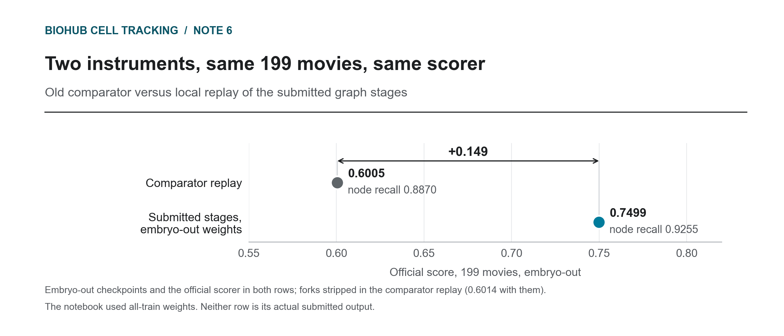 Figure 1. Local replays on the same 199 movies with embryo-out backbone weights. Reproducing the submitted graph stages raised score from \(0.6005\) to \(0.7499\). The actual notebook used all-train weights, so this was not a measurement of its output.
Every verifier threshold, deletion rule and association arm of the preceding weeks had been chosen on the comparator replay’s lower-recall graphs. The two local replays differed even before changing the evaluation population. Their \(0.149\) gap showed why a low local score could not be attributed entirely to unseen-embryo difficulty.
The replay provided a common reference after seven baselines had been used since Note 3 (the \(0.6014\) of Section 0 is the same comparator with the old forks left in; Note 4’s research replay, base near \(0.74\), is another graph family), and levels are quoted on it from here on.
There, with the notebook’s raw forks collapsed, the base is \(0.7489\), and every division number below is measured over it. A label oracle over this replay’s candidates scores \(0.8007\) at division Jaccard \(0.5097\) (\(79\) true positives, \(4\) false, \(72\) missed). The 72 missed events had no candidate row at all. Roughly half the annotated divisions were therefore outside the generator’s reach before ranking; their upstream causes had not yet been measured.
3.3 What the Replay Did Not Explain
On the replay’s graphs the deployed verifier drew \(2\) true and \(3\) false divisions, a local division Jaccard near \(0.013\), below the \(0.062\) of the comparator replay. Correcting the replay did not reconcile the local division result with the conditional estimate near \(0.32\). Population differences and the unmeasured hidden edge contribution remained unresolved. The replay did expose a fixable problem: the verifier had been fitted on the old pipeline’s candidates and was being applied to the submitted pipeline’s. Clause C12 follows: validate on the pipeline that ships.
4. Rebuilding on the Submitted Pipeline: the Refit and v83
The fitting mismatch predicts that a verifier fitted on the submitted pipeline’s own candidates should do better on its graphs than one fitted on the old ones. The test held those graphs fixed and changed only the fitting candidates.
Fits compared on the deployed-stack replay: 199 movies, embryo-separated ranker fits, fork-free base 0.7489.
| Verifier training table | Delta over base | Division TP / FP |
|---|---|---|
| deployed verifier, fitted on comparator-replay candidates | +0.0013 | 2 / 3 |
| refit on the submitted pipeline’s candidates only | +0.0030 | 5 / 13 |
| refit on the union of both tables | +0.0065 | 17 / 90 |
The prediction held. The deployed selector gained \(+0.0013\), compared with \(+0.0065\) for the tested union refit, and fired nothing across the larger embryo’s \(128\) movies. Ranker fitting was split by embryo, but its training and runtime candidates came from different pipelines.
I selected the union fit: its sweep was a plateau, and both embryos were positive at the peak (\(+0.0096\) and \(+0.0060\)). Translating it to the runtime replaced per-embryo thresholds with one flat threshold chosen by a rule fixed in advance. The kernel passed its hold-in gate on the four example movies with nearly unchanged edge counts: \(2028/155/99\) true/false/missed against \(2027/155/100\).
v83 was the refit’s sanity check, with its reading written down before submission:
1
2
3
>= 0.940       the refit transfers; make it the base
0.937 - 0.939  neutral; the refit is not distinguishable
< 0.937        the flat threshold hurt; revert to per-embryo
It returned \(0.944\), \(+0.007\) over v80’s \(0.937\) (the reference for the bands) and inside the band for making the refit the base: no failure detected, so the refit became the base.
These deltas have different comparators: the local \(+0.0065\) (and Section 5’s corrected \(+0.0046\)) uses a fork-free graph, while the Public \(+0.007\) compares against v80, which already had a verifier. I nevertheless expected later division gains to transfer similarly, an extrapolation from the few submissions available.
5. The Shipped Code as the Validation Tool
On 2026-09-03 a parity check asked the same question one level down, comparing the shipped runtime module inside the kernel with the same division-stage recipe run locally: on the four example movies the kernel applied \(50\), \(23\), \(3\) and \(50\) divisions, and the local recipe applied none.
The cause was a flag: every local rebuild of the division tables had generated candidates only around annotated sources, since only annotated regions produce labels. On one example movie that yields \(7{,}519\) rows; the shipped runtime, which does not know where the annotations are, generates \(358{,}000\). The local sweep omitted much of the runtime candidate population. Its chosen threshold and budget therefore needed evaluation on the complete runtime-generated graphs, including any additional scored false positives.
The fix follows C12: the shipped runtime module itself became the selection tool, and rebuilt tables became training material only. Re-run that way, the deployed operating point was the best eligible setting in the tested sweep: \(0.7535\) against the fork-free \(0.7489\), \(+0.0046\) with both embryos positive, and no threshold or cap change cleared the rule written down for a new operating point.
The sweep also showed why a large number of added forks need not produce many scored division errors. Under sparse annotation, a structurally valid fork without evaluable ground-truth context may be ignored. An unmatched parent does not guarantee exemption: the patched scorer also counts invalid forks, including cross-component and malformed branches identified through their descendants.
The all-train, in-sample run applied \(4{,}662\) divisions and counted \(71\) false positives and \(42\) true positives. In the embryo-out arms, caps spanning a factor of four scored \(0.7536\), \(0.7535\) and \(0.7535\). Most extra picks did not change the scored counts in these runs. Only \(8\) of \(79\) reachable divisions were recovered, directing the next experiment toward ranking. The corresponding hidden TP/FP counts were unavailable.
6. Three Older Levers, Retested on the Submitted Pipeline
6.1 A Joint Lineage Action and Its Folds
A composition that scores parent-and-children decisions jointly, the project’s most-cited undeployed gain, measured \(+0.0187\) on the deployed-stack replay, positive on both embryos. A fold audit then found its heads had been trained on four folds that each held movies from both embryos, the defect Note 4 took apart.
The two head constructions are compared on the same 199-movie deployed-stack replay.
| Head training split | Pooled | 71-movie embryo | 128-movie embryo |
|---|---|---|---|
| folds mixing both embryos | +0.0187 | +0.0152 | +0.0191 |
| embryo-disjoint folds | +0.0004 | +0.0150 | -0.0021 |
The head trained on the 128-movie embryo transfers; the head trained on the 71-movie embryo does not. With no third embryo, too few movies and poor generalization cannot be told apart. I stopped these head configurations because they failed the rule requiring a non-negative change on both embryos.
6.2 Line-Fit Smoothing, Sub-Voxel Coordinates and the Rules
On September 1, adding interior line-fit smoothing to the old local replay moved \(0.6005\) to \(0.6192\), a gain of \(+0.0187\). This happens to equal the joint lineage-action gain in Section 6.1, but came from a separate experiment on a different comparator. The deployed notebook already included line-fit smoothing, so the proposed v82 applied it a second time and failed its hold-in gate. The September 3 audit explained why the earlier local gain was not an improvement available to that notebook.
Remeasuring line-fit on the deployed-stack replay exposed a different cost. The kernel smooths positions along short track segments and then writes integer voxel coordinates. Quantizing \(4.75\) million smoothed positions cost \(0.0050\), with both embryos losing (\(-0.0005\) and \(-0.0057\)). A kernel writing three-decimal coordinates ran clean but was not submitted: the competition’s Evaluation page specifies integer centroid coordinates in voxels.
The hold-in check moved the other way (\(2024/157/103\) against \(2028/155/99\)). Different peak-location errors were one possible explanation, but the checks also used different weights and evaluation populations. Those counts alone could not identify the cause of the reversal.
6.3 A Deletion Rule That Changed Sign With the Pipeline
The last cheap post-processing rule deleted nodes whose incident edges all carry low probability. It had measured \(+0.0009\) on the comparator replay; on the deployed-stack replay it measured \(-0.0106\) at the same setting, and its best variant was a literal no-op. On the submitted pipeline, edge probabilities come from a different fusion of the two detectors’ scores, and several stages add edges with probability exactly zero, so “all incident probabilities are weak” can also select real cells in difficult regions.
7. The Detector Tail, Tested on the Rebuilt Validation
7.1 Why I Investigated the Low-Recall Movies
On the deployed-stack replay, per-movie adjusted edge Jaccard correlates \(0.82\) and \(0.79\) with node recall in the two embryos, and lifting only the worst decile of each embryo to its median is worth \(+0.0277\) and \(+0.0233\): this identified a consequential low-score subset. The hypothetical median replacement did not establish that it contained all remaining improvable errors. In the twelve worst and twelve median movies, miss rates were \(36.5\%\) and \(4.6\%\).
| tercile, worst twelve movies | low / mid / high |
|---|---|
| miss rate by intensity at the ground-truth position | 0.579 / 0.324 / 0.192 |
| miss rate by local predicted-node density | 0.653 / 0.272 / 0.109 |
Misses concentrate where the scene is sparse, graded by brightness. In the worst twelve, \(48\%\) of misses are invisible in the detector’s own field (the neighborhood-maximum logit at the ground-truth position is below zero), a limitation of the current detector output; in the median twelve, \(62\%\) are above threshold but absorbed by a neighboring peak, an inference-time one. The other embryo’s tail movies have raw detector recall of \(0.987\) and lose their cells later, in association and the solver.
7.2 Intensity Augmentation Improved Recall on the Selected Tail
The trainer had no intensity augmentation, and the brightness-related failure pattern motivated an intensity-augmentation test; it did not by itself establish domain shift as the cause. I added one (gamma, global gain, a smooth regional-dimming field, an additive haze floor and per-voxel noise), with go conditions written before any candidate existed. At epoch ten, on the larger embryo’s worst seven movies, raw node recall went from \(0.7123\) to \(0.8884\) and the invisible share of misses from \(0.706\) to \(0.198\). Peaks per estimated cell also rose, from \(1.701\) to \(2.10\) on the tail.
7.3 Evaluating the Detector in the Complete Pipeline
The detector was then evaluated in the deployed pipeline under the official metric, embryo-out, on \(15\) movies of the larger embryo: the seven worst and eight near the median.
| Composition | Worst 7: delta | Median 8: delta | Median movies harmed |
|---|---|---|---|
| primary detector, deployed threshold | +0.1007 | -0.0198 | 5/8 |
| primary detector, strict threshold | +0.0583 | -0.0169 | 5/8 |
| detection-only third field, lower weight | +0.0124 | -0.0073 | 5/8 |
| novel-peak union, strict threshold | +0.0417 | -0.0306 | 8/8 |
| hole-filling union, sparse regions only | +0.0448 | -0.0175 | 6/8 |
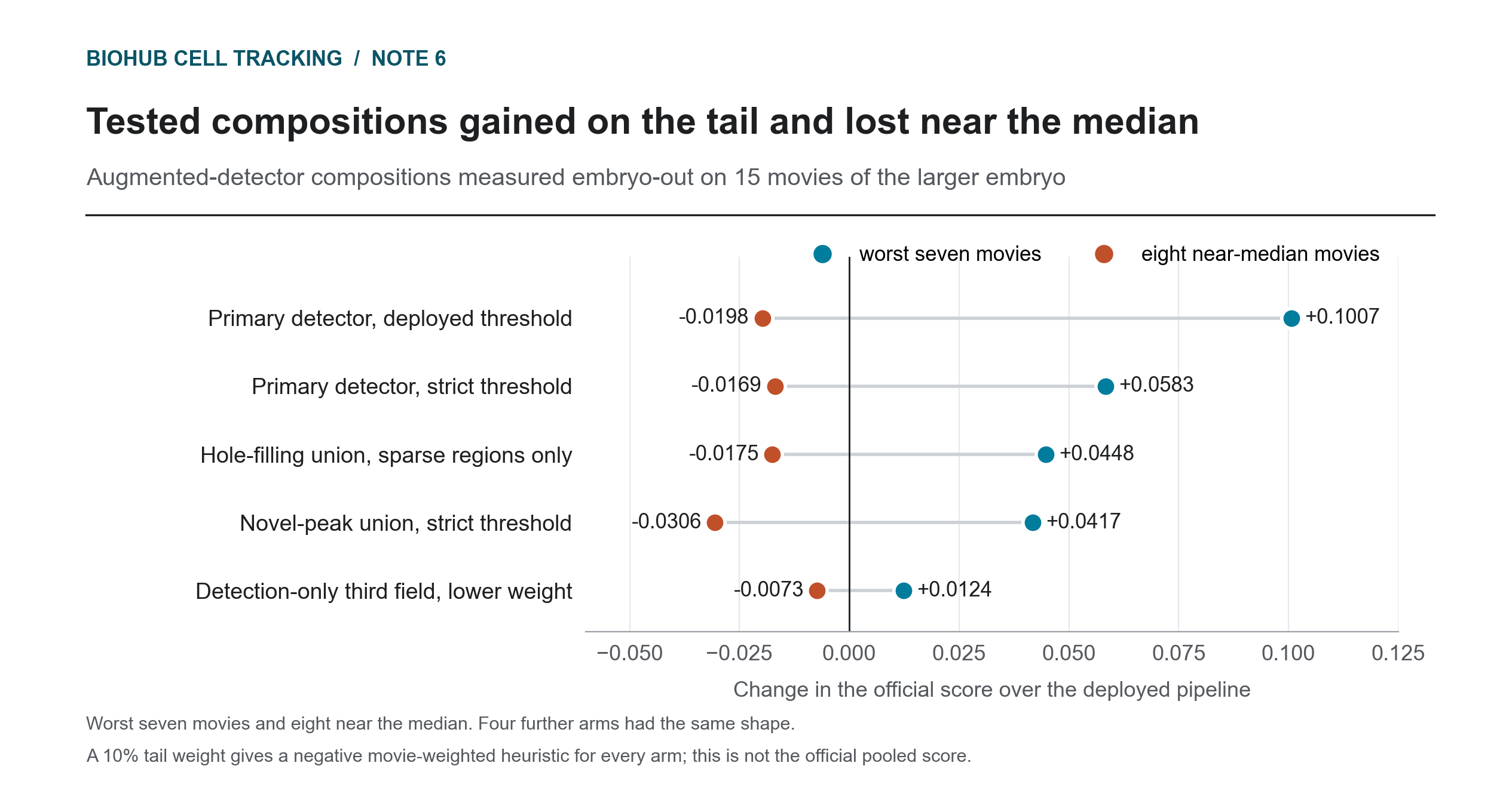 Figure 2. Every composition gained on the worst seven movies and lost on the eight near the median. A simple mixture weighted by movie count was negative for every arm. It is a screening heuristic, not an estimate of the official aggregate, whose edge and division weights differ.
Four further arms had the same shape; every arm paired the augmented first split with a deployed second split (the augmented pair was never trained). On the worst movie the official adjusted edge Jaccard went from \(0.248\) to \(0.487\), but every tested composition also lost on the median movies. A movie-count mixture with tail share \(\pi \approx 0.10\) put the values between about \(-0.005\) and \(-0.025\). This was only a screening heuristic: the official score pools edge denominators and division counts separately, so subgroup score deltas cannot generally be averaged with movie-count weights. It also assumed the selected movies and tail share represented the target population.
Added objects and the count adjustment. The metric scales each movie’s edge Jaccard by \(1-0.1\,r_i\), where \(r_i\) is the relative excess of predicted nodes over a supplied coarse cell estimate, so a movie just under the estimate earns a small bonus and one just over pays a penalty. On one median movie estimated at \(5{,}257\) cells, the hole-filling arm took the node count from \(5{,}047\) to \(5{,}439\) and the score from \(0.7735\) to \(0.7050\), while node recall rose only from \(0.9915\) to \(0.9957\): about twenty more annotated cells for \(392\) added nodes. Holding edge Jaccard fixed and assigning the entire starting score to the adjusted edge term gives a count-only loss of about \(0.0058\). Any positive division contribution makes that estimate smaller. Count adjustment alone therefore cannot explain the observed \(0.0685\) loss; crossing the estimated count is not a discontinuity in the formula.
Losses with nearly unchanged node counts. In the gentlest arms one movie went from \(0.767\) to \(0.722\) at \(+0.2\%\) nodes: a nearly unchanged total node count can still hide changes in peak identity, position and graph connectivity. This observation alone does not attribute the loss to sub-voxel displacement. Raising the extraction threshold halved the tail gain and barely changed the median loss, so that threshold change did not resolve the composition problem. A control on 2026-09-04 with an ordinary third seed in the detection-only role lost \(-0.0063\) on the same median eight (\(6\) of \(8\) negative), close to the augmented model’s \(-0.0073\): the similar losses suggest that adding a third field mattered, but do not provide a causal decomposition of augmentation and mixing.
7.4 Why the Program Was Closed
A subgroup fix needs a usable test-time routing signal. Frame contrast and novel-peak fraction did not separate the low-recall and median-movie panels. Because every tested composition harmed the median panel, I stopped this experiment. A wider router search and the official aggregate effect on a representative population remained untested.
Closing
The investigation found two mismatches: the comparator replay built different graphs from the notebook, and the local verifier sweep generated candidates only near annotations. Replaying the submitted stages and the complete runtime candidate population changed which modifications were worth pursuing. A verifier refit on the new candidates became v83.
The hidden division counts remained unknown. Locally, the verifier still recovered few reachable divisions, so I began labeling its candidates. The first \(69\) judgments moved the runtime replay from \(0.7535\) to \(0.7547\). The next question was whether replaying the submitted pipeline was enough to judge a change under hidden-test conditions.
Decision record, evolving criteria and remaining questions
The tables below retain the period’s decisions. The clauses summarize the scope of the evidence; their presence does not certify that every earlier experiment satisfied them.
8. Decision Log
The rule in force was the two-fold embryo-disjoint out-of-fold replay over the 199 training movies, both embryos non-negative; the week moved it from the comparator replay onto the deployed-stack replay and the shipped runtime module. Three submissions went out. v80 tested a locally chosen operating point with a written expectation of \(0.937\); v81 removed fork application to measure the package effect (Section 2). v83 then checked the locally chosen refit.
| decision | reason at the time | what came back | what it changed |
|---|---|---|---|
| six bets on named bottlenecks (Section 1) | verifier gain was a tenth of the label-assisted diagnostic; about 80 positives | no verifier gain; detector trainer +0.0466, pipeline -0.0272 | these six configured interventions did not advance |
| v80 operating-point check and v81 stage removal (09-01) | test the local sweep choice; use removal to estimate the hidden division contribution | Public package effect +0.032; division Jaccard near 0.32 only if hidden edge change is negligible; v80 a tie | C13; the gap pointed at the local evaluation |
| deployed-stack replay (09-02) | the conditional division estimate; the untested 0.60 against 0.94 gap | 0.7499 against 0.6005, same movies and scorer | C12; one reference for levels (C5) |
| refit on the submitted pipeline’s candidates; v83 as its sanity check (09-03) | the deployed verifier, fitted on the other pipeline’s candidates, drew 2 TP and 3 FP | local +0.0065, both embryos positive; Public 0.944, in the “make it the base” band | the refit became the base |
| shipped runtime as the selection tool (09-03) | the local recipe applied no divisions where the kernel applied dozens | deployed operating point best among tested settings, +0.0046; caps do not bind | rebuilt tables are training material only |
| re-measure three earlier modifications | each had a positive earlier measurement | JLA +0.0004 embryo-disjoint; line-fit already deployed (v82 doubled it); rounding cost 0.0050 but integer output required; deletion -0.0106 | all three closed without a submission |
| detector-tail program (09-04) | the selected low-recall movies had brightness-related misses | tail recall 0.7123 → 0.8884; every composition lost on median movies | closed for lack of a router; I began hand labeling |
The criterion at the end of this period
| clause | wording | since |
|---|---|---|
| C1 | Separate fitting, calibration and evaluation dependencies, and score the whole graph; movie separation alone does not ensure domain independence | Note 2 |
| C2 | Write each gate down before the result exists | Note 3 (07-15) |
| C3 | Calibrate a rule on the population it will act on | Note 3 |
| C4 | Judge a component by the graph it produces, in an exact replay, not by its own accuracy | Note 3 |
| C5 | Bind every level and delta to its comparator; do not rank deltas from different replays; the deployed-stack replay becomes the reference here | Note 3 |
| C6 | A candidate must finish on the hidden set within the time limit | Note 3 |
| C7 | Folds hold out a whole embryo (embryo-out) | Note 4 |
| C8 | Numbers from movies the deployed model trained on (hold-in) are not evidence of generalization | Note 4 |
| C9 | Use the board for matched sanity checks with a written expectation, not to choose adjacent settings | Note 4 (08-10) |
| C10 | Measure candidate reach; call a diagnostic a bound only within its declared scope | Note 5 |
| C11 | A gate must be able to end in a decision | Note 5 |
| C12 (new) | Validate on the pipeline that ships: replay it exactly | Note 6 |
| C13 (new) | Use a stage-removal probe to measure its package effect; isolating a metric term needs extra assumptions | Note 6 |
9. What the Period Established
Established
- v79 − v81 measured a \(+0.032\) Public package effect. Division Jaccard near \(0.32\) is conditional on negligible hidden edge change; local division Jaccard was \(0.062\).
- On the same 199 movies and scorer, the comparator replay scored \(0.6005\) (node recall \(0.8870\)) and the deployed stack \(0.7499\) (\(0.9255\)).
- On identical graphs from the submitted pipeline, the union refit gave \(+0.0065\) against the deployed selector’s \(+0.0013\), and \(+0.0046\) (\(0.7535\) over \(0.7489\)) through the shipped runtime, both embryos positive.
- A valid fork without evaluable annotated context may be ignored, but unmatched parents do not exempt invalid cross-component or malformed forks. Only \(8\) of \(79\) reachable events were selected locally; the hidden false-positive cost was not measured.
- On the submitted pipeline, \(72\) of the \(151\) annotated division events have no candidate at all.
- External detector data read \(+0.0466\) on trainer validation and \(-0.0272\) through the deployed pipeline on two movies.
- With embryo-disjoint heads, the joint lineage action gives \(+0.0004\) where mixed folds gave \(+0.0187\).
- Intensity augmentation raised raw recall on the larger embryo’s seven worst movies from \(0.7123\) to \(0.8884\), and every evaluated composition lost on typical movies.
Supported but Unconfirmed
- That the smaller embryo’s head transfers poorly because of training-set size rather than embryo difficulty.
- That a fully augmented detector pair would behave like the tested augmented first split.
Open Questions
- How much of the Public stage-removal difference came from division Jaccard and how much from adjusted edges?
- Would another locally selected division change pass a matched Public sanity check?
- Can ranking at annotated parents improve through a signal other than new labels?
- Is there a usable test-time router beyond the two statistics examined?
- Would training to preserve peak positions avoid the composition loss?
Series: