BioHub Cell Tracking Working Note 7: When the Same Code Was Not the Same Experiment
Series links and references
- Competition: BioHub - Cell Tracking During Development
- Official metric notes: RoyerLab kaggle-cell-tracking-competition metrics.md
- Previous notes:
- Working Note 1: Learned Lineage Graphs and Metric-Aware Repair
- Working Note 2: From a Leaderboard Plateau to OOF Structural Diagnostics
- Working Note 3: What the OOF Machine Refused
- Working Note 4: Three Gaps in Local Validation
- Working Note 5: What a Frozen Graph Left Untested
- Working Note 6: When Local Validation Ran a Different Pipeline
- Korean version: BioHub Cell Tracking 작업 기록 7: 같은 코드로도 검증이 어긋나는 이유
- Follow-up: BioHub Cell Tracking Working Note 8: What Went Into Choosing the Final Two
Related public notebooks
About this series. BioHub asks competitors to reconstruct cell lineage graphs from 3D microscopy movies. The labeled training set contains 199 movies from two embryos; Public scores cover 29% of the hidden test set, and Private scores cover the remaining 71%. The hidden test comes from embryos not seen in training. Each note follows the record through its stated period; later findings and retrospective comments are marked separately.
Note 6 left a question: is replaying the submitted pipeline enough to judge a change under hidden-test conditions? Between September 5 and 12, hand labels improved the 199-movie graph score by \(+0.0048\), but the submitted package lost \(0.005\) on Public. A pseudo-label detector gained \(+0.0423\) when blended with an embryo-out primary, while its all-train deployment scored \(0.924\).
The labels raised questions about precision and annotation conventions. For the detector, running the shipped weights exposed a destructive alignment step. A teacher-clean control also failed to reproduce a useful pseudo-label composition. The comparisons depended on the weights, candidate population, labels and teacher training path, as well as the code.
0. Where the Week Started: Validation Rebuilt on the Submission Pipeline
The pipeline is Note 6’s. A detector scores every voxel of each 3D frame, and the peaks become candidate nuclei; a secondary detector’s field is aligned to the primary’s and blended in first. A transformer scores links between frames, an integer linear program (ILP) selects a consistent graph, and a gradient-boosted division verifier, retrained inside the notebook from a shipped table of labeled candidates, decides which candidate divisions to add. The kernel is the submitted Kaggle notebook; the hidden set is the test movies behind the board.
The \(199\) training movies come from two embryos, of \(128\) and \(71\) movies (the larger and the smaller embryo); embryo-out means trained on one and scored on the other. The main local instrument is the deployed-stack replay, which the project called kernel-faithful: the shipped runtime code run over all 199 movies with embryo-out models, scored by the official scorer, each embryo reported separately. The four example movies with public labels are copies of training movies, so scoring the deployed models on them is hold-in: it can catch damage but cannot select.
The deployed kernel entering 2026-09-05 was v83: \(0.7535\) on the deployed-stack replay, with \(8\) true and \(19\) false divisions locally, and \(0.944\) on the board.
1. The First Idea: Hand Labels for the Division Verifier
Note 6 had found the division channel limited by the verifier’s ranking; a ranker learns from labeled examples, so more correct labels should give it more to rank with.
1.1 What the Labels Bought Locally
Each labeling item showed one candidate division from a training movie, and I answered yes, no or skip; unmarked gold rows, whose answer the annotation already fixes, measured my agreement. The first \(250\) items (\(14\) of \(16\) gold rows correct) added \(58\) positives, \(232\) in total.
Verifier tables compared on the 199-movie deployed-stack replay.
| Training table and threshold | Score | Division TP / FP |
|---|---|---|
| deployed table, threshold 0.75 | 0.7535 | 8 / 19 |
| +58 hand positives, threshold 0.75 | 0.7573 | 19 / 71 |
| +58 hand positives, threshold 0.65 | 0.7583 | 24 / 96 |
Both embryos rose in both arms (overall \(+0.0038\) and \(+0.0048\)), and kernel v85 shipped the higher-scoring \(0.65\) arm. False positives rose from \(19\) to \(96\), yet the simultaneous TP increase outweighed them in the local score (Section 1.3).
1.2 The Sanity Check on Public
The Public sanity check tested the local decision on unseen embryos. Its reading was written before the score: \(0.947\) or more would support the labels, \(0.944\) to \(0.946\) would be neutral, and below \(0.944\) would mean the hand rows or the lower threshold hurt. It returned \(0.939\), a loss of \(0.005\) and below the adverse line written for that submission. It also lies outside the \(\pm0.002\) tie band formalized on September 5–6 (Section 3). The band was a project reading rule, not the mathematical resolution of the rounded score.
On the four example movies, which hold only three annotated divisions, v85’s edge counts were exactly v83’s. That made hidden division precision a plausible explanation, without measuring either hidden metric term.
1.3 A Possible Precision Mismatch
The official score is a node-count-adjusted edge Jaccard plus the division Jaccard at weight \(0.1\), the division term counted over all events together (TP matched divisions, FP forks counted as false by the scorer, FN missed annotated divisions):
\[J_{\mathrm{div}}=\frac{TP}{TP+FP+FN}.\]For additions that leave existing event matches unchanged, recover missed true divisions, and add counted false divisions, the division term improves when the added precision exceeds \(J_{\mathrm{div}}/(1+J_{\mathrm{div}})\). This calculation holds the rest of the graph fixed. A real fork edit can also alter matching and edges, so the condition alone does not predict its total score effect. Locally the term is dominated by misses: \(J_{\mathrm{div}}\) sat between \(0.06\) and \(0.10\), with \(127\) of \(151\) events missed, so its break-even precision was low, but not zero. Note 6’s probe would imply hidden division Jaccard near \(0.32\) only if the hidden edge effect were negligible. The following calculation explores that hypothetical starting point.
Start with hypothetical counts of 32 TP, 20 FP and 48 FN, giving \(J=0.32\). The local additions had precision \(p=16/(16+77)\approx0.172\). At the same precision, recovering 8 more true divisions would add about \(8(1-p)/p=38.5\) false divisions. Jaccard would fall to \(40/(40+58.5+40)\approx0.289\), a weighted score change of about \(-0.0031\) if edges stayed unchanged. A larger loss near \(-0.01\) would require worse precision: for example, 80 extra FP for the same 8 TP would give \(40/(40+100+40)\approx0.222\).
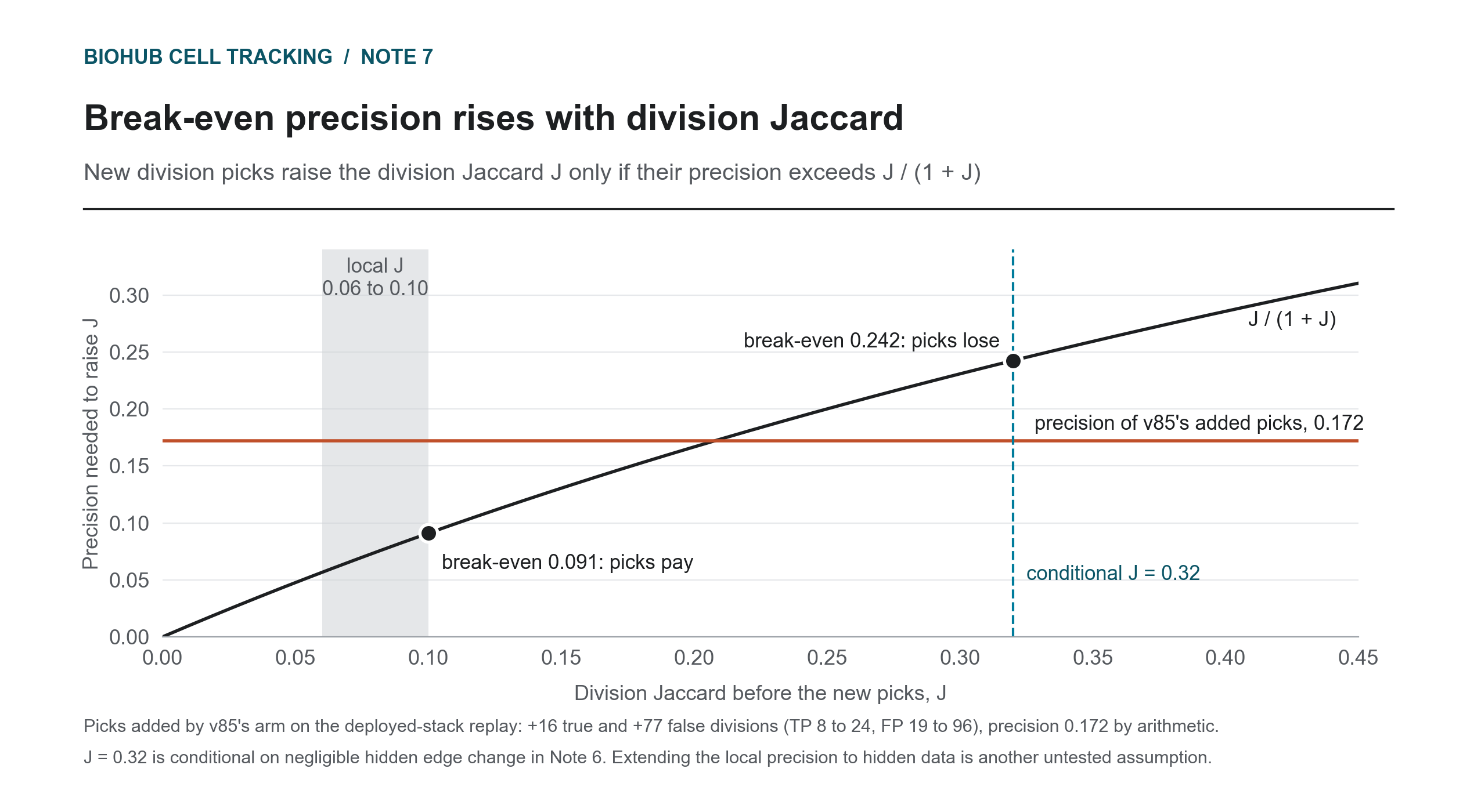 Figure 1. Sensitivity to the starting division Jaccard when existing matches stay unchanged. The local added-pick precision clears the threshold at the local Jaccard, but not at the hypothetical \(J=0.32\).
A related local observation was that candidates in the score bands from \(0.65\) to \(0.85\), where most of v85’s additions sat, were true only \(13\) to \(29\%\) of the time.
Two things changed. Division operating points moved to the precision frontier: false positives near v83’s level, and the most true positives at that level. And I withdrew Note 6’s working expectation that division changes are not damped on the hidden set: v85 was the first division change whose local gain came back negative on the board, so the expectation had rested on a few observations, not a rate.
2. Tracing the Failure: Precision First, Then the Labels Themselves
2.1 A Second Batch, at the Precision Frontier
If false divisions were the loss, the labels could still help at a stricter operating point. A second batch of \(500\) items gave \(253\) positives, and v86 shipped them at threshold \(0.90\), scoring \(0.7591\) locally with \(18\) true and \(25\) false divisions. A simple heuristic favored v86: it weighted added forks by the precision of my labels in each score band (\(2{,}324\) picks at an estimated \(0.825\), versus \(2{,}242\) at \(0.41\) for v83). That estimate described my candidate judgments, not the scorer’s matched events. It could motivate the test but could not predict official Jaccard without knowing which forks would count. The board returned \(0.943\), a tie with v83, the kernel without hand labels: most of v85’s loss was gone, and no gain showed. v85 and v86 had each changed the label table and the threshold together, so neither reading can say which change did what (clause C16).
2.2 Measuring the Labeler Against the Scorer’s Convention
The gold rows raised a question about the labels themselves: I had answered “no” to roughly \(15\%\) of the annotated divisions, so I measured how the ground truth places all \(151\). At the annotated parent frame, \(75\%\) show exactly one detection within \(7\,\mu\mathrm{m}\) of the parent, \(15\%\) show two and \(8\%\) none: the annotation puts the division edge where the parent is still one nucleus, and the daughters appear one frame later, a median \(10\,\mu\mathrm{m}\) apart against \(8.7\,\mu\mathrm{m}\) for my own positives.
In all seven gold divisions I had rejected, the annotated daughters sat on our candidate pair. I re-judged the rejected items whose daughters were at least \(9\,\mu\mathrm{m}\) apart (\(99\) and \(109\) from the two batches) under the annotation’s convention. Sixty changed from no to skip, and none became yes: cells appearing from behind, divisions into depth, which as “no” labels had taught the verifier to reject candidates the annotation may count.
Simply combining these batches did not help: their union scored below the second batch alone in the local comparison. Whether the mismatch explains v85 and v86 on the board is an untested hypothesis. The code and scorer were aligned, but my labeling convention had not been checked against the scorer’s event definition. That became C17: check what a human label means before using it to train or select a model.
3. Isolating One Change: v87 and the Selection Rule
v87 changed one thing: it kept v86’s table and threshold and changed only the verifier’s runtime features. The three new features encode cues I used when labeling: the distance to the nearest detection at the daughter’s position one frame early, and the brightness there over two frames. Locally it scored \(0.7609\) with \(23\) true and \(40\) false divisions; its reading was written before it ran.
Before v86’s score existed, I had set a condition for that night: submit v87 if v86 reached \(0.945\) or more, not if it read \(0.944\) or less. v86 read \(0.943\), \(0.001\) from v83 on Public’s \(29\%\) share of the test, so the condition would have let a tie decide whether an experiment ran; and v87’s question did not depend on v86’s level, since v86 was its control in the program’s only single-change comparison. I set the condition aside after its input was known and submitted v87.
v87 returned \(0.946\): \(+0.003\) over v86, at the project’s threshold for investigating a Public difference, and a tie with v83. If that single-axis step is real, it belongs to the runtime features, which locally did nothing without the labels (\(0.7489\) on the old table, no true divisions).
The written rule of 2026-08-28, a response to a long stall, still named the board as the objective, though every selection of the previous week had been made locally. Over 2026-09-05 and 2026-09-06 I rewrote it:
1
2
3
4
5
6
select on leakage-safe local evidence: embryo-out, kernel-faithful,
  both embryos non-negative, division operating points on the precision frontier
a Public difference within 0.002 is a tie
the board is cited only to falsify a large move (about 0.003 or more)
submit only hypotheses written down before the result exists
never rewrite a rule after a score
Two of its lines come from the v87 night: no gate should take a board difference within \(0.002\) as its input, and a written gate is not rewritten after a score. There were no submissions between v87 and 2026-09-10.
4. Three Questions Local Validation Settled Without a Submission
On 2026-09-06 I wrote a plan with four lanes, each with a gate written before its first number: graph-stage constants, rival-parent features for the division verifier, a division-aware fine-tune of the association head, and a detector trained on our own tracks (Section 5). The first three concern mechanisms the replay measures directly; each closed within two days on its own gate.
The association head missed its discrimination gate. The AUC of the deployed heads’ score margin between the two cases was \(0.610\) and \(0.683\), against a gate of \(0.70\); a head trained with more than ten thousand real zebrafish divisions reached \(0.643\), no better. The lane closed within hours of its pilot.
Rival-parent features did not improve the runtime verifier enough. A three-feature logistic separated captured daughters with an embryo-out AUC of \(0.80\), but inside the runtime at \(0.90\) the verifier scored \(0.7599\) with \(21\) true and \(39\) false divisions, against \(0.7605\) with \(23\) and \(47\) for the shipped features, far from its shipping rule. At the time I read these failures as saturation of the available geometry and appearance signals and looked upstream. That interpretation was broader than the tests: they had stopped these configured features and rankers, not every way to represent division evidence.
No tested graph constant cleared the required gain on both embryos. After fixing a bug that had silently ignored environment overrides in the replay, none of fourteen arms on twelve diagnostic movies passed the both-embryo rule. Lowering the edge threshold from \(0.50\) to \(0.35\) gave \(+0.0646\) on the smaller embryo and \(-0.0117\) on three movies of the larger, the node-to-estimate ratio rising from \(1.056\) to \(1.146\): the threshold drops edges before the ILP, which then deletes disconnected nodes, and lowering it kept real cells on the smaller embryo and over-detections on the larger. At \(0.45\), all 199 movies gave \(+0.0081\) and \(+0.0008\) against a rule of \(+0.003\) on both, and I closed the lane.
5. The Second Idea: Positive Labels for Unannotated Nuclei
5.1 The Hypothesis
The September trainer marks annotated nuclei as positive and other voxels as negative, with a negative-loss weight of \(0.01\). Annotations covered about \(2.8\%\) of the estimated cell population. Pseudo-labels could therefore add positive supervision where most nuclei had only a downweighted negative target. Pseudo-labels are labels produced by a model; here, our own embryo-out tracks, which added to the ground truth gave \(36\times\) more labeled nodes from the same domain (\(4.76\) million against \(133\) thousand). The model whose tracks became labels is the teacher; the detector trained on them is the student. I expected the ILP to prune the student’s extra peaks.
The leak argument, written before the first number, was that the student never trains on the embryo it is scored on. Beside it sat a caveat, with a control planned: the tracks on the student’s training embryo came from a teacher trained on the embryo the student is scored on, so part of any gain could be that embryo’s annotations distilled back through the teacher.
5.2 The Gates, and Two Clauses I Rewrote
| student as primary, embryo-out | Tail: mean adjusted-edge Δ | Typical: mean adjusted-edge Δ |
|---|---|---|
| epoch 10, as primary, 15 larger-embryo movies | +0.1280 | +0.0307 |
| epoch 50, as primary, same movies | +0.1358 | +0.0774 |
| reciprocal student, as primary, 9 smaller-embryo movies | +0.1124 | +0.1033 |
Tail movies are where the deployed pipeline scored worst, typical movies sit near the median, and the reciprocal student was trained the other way round. The first row’s pass rule, written in advance, asked for at least \(-0.003\) on typical movies and \(+0.03\) on the tail; its \(+0.0307\) is the rounded \(+0.031\) headline: the mean adjusted-edge gain on the eight typical movies in the 15-movie primary-detector panel (mean total-score gain \(+0.0293\)). It was my first detector gain on typical movies, where Note 6’s augmented detector had lost.
Two clauses written in advance failed, and I changed both. The reciprocal rule capped the pooled node-to-estimate ratio at the base plus \(0.05\), and it rose from \(1.027\) to \(1.201\); before the 199-movie numbers existed, I replaced the cap with \(+0.003\) on both embryos, a score that already includes the count penalty, plus a cap of \(1.5\) on each embryo’s median per-movie node ratio. A later composition rule allowed the six smaller-embryo movies that had lost most as primary to lose at most \(0.02\); they lost \(0.0257\), and after that number was known I waived the clause and left the decision to the 199-movie run, whose rule was already written. Both changes loosened a gate toward shipping, the direction C2 guards against, and both stay in the record.
5.3 From 199 Movies to a Kernel
The composition carried forward used the student as the secondary detector, beside the replay’s embryo-out primary. On all 199 movies it moved the official score by \(+0.042302511\), with both embryos positive; forty-three movies fell, including \(17\) of \(28\) high-base movies of the smaller embryo (base score at least \(0.85\)), a slice written down before any submission.
Kernel v88 swapped the secondary weights for an all-train student, selected at about epoch \(52\) by a trainer proxy on \(40\) training movies, and carried two small validity repairs: a guard against an added division giving a cell a third child, and integer output coordinates kept inside the volume. The all-train student that v88 loaded was never scored anywhere; every 199-movie number came from the embryo-out pair. The leak control had not yet run. v88’s reading, written before its score, called \(0.943\) or less materially adverse and \(0.949\) or more support.
6. The Sanity Check Fails: Validation Never Ran the Shipped Weights
v88 returned \(0.924\), \(-0.022\) against v87, far below its adverse line, with every local gate, as rewritten in Section 5.2, passed.
6.1 One Alignment Formula
A detector’s raw output for each voxel is a logit, strongly negative where it sees background and positive where it sees a nucleus. The kernel aligns the secondary’s logit field to the primary’s, then blends them before peak extraction:
\[A=\left(S-\mu_S\right)\operatorname{clip}\!\left(\frac{\sigma_P}{\sigma_S},\,0.5,\,2\right)+\mu_P, \qquad B=0.525\,P+0.475\,A,\]where \(P\) is the primary’s field, \(S\) the secondary’s, and \(\mu\), \(\sigma\) are taken over the whole frame.
The formula treats differences in whole-frame mean and spread as calibration differences. Dense pseudo-label training also changes how much foreground a detector predicts, so this correction can move real peaks along with the background. On a bright example movie, the kernel’s primary, an older all-train model, averages \(-14.7\) over the frame. The student, trained on dense pseudo-labels, fires on \(10\) to \(16\%\) of voxels against \(3\%\) for the primary, and averages \(-5.0\): its whole-frame mean is about ten higher. Different foreground coverage and background logits can both affect that mean. Sliding it down by about ten drags its real peaks below the threshold too (Figure 2).
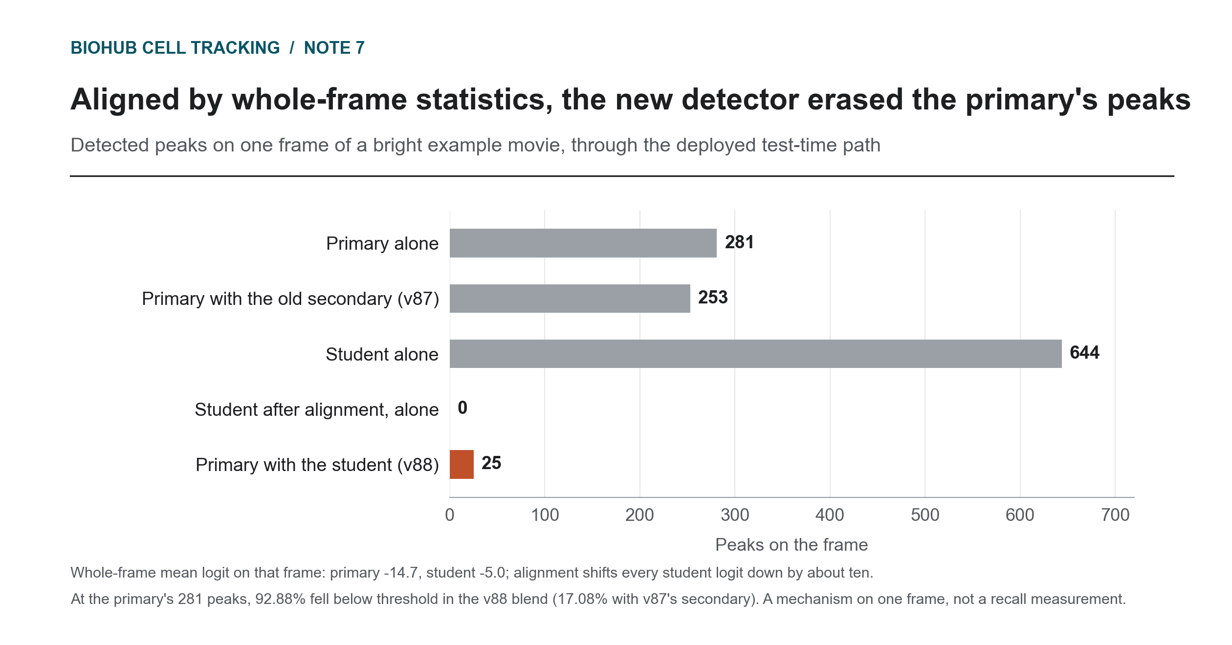 Figure 2. Peaks on one frame of a bright example movie, through the deployed path. Aligned by whole-frame statistics, the new detector left \(25\) peaks where the primary alone had \(281\). This is a mechanism on one frame, not a recall measurement.
6.2 Why Local Validation Could Not See It
The deployed-stack replay runs the deployed code with embryo-out weights, whose primaries sit at mean logits of about \(-6\) to \(-9\); in those tested compositions the aligned student added recall. That did not guarantee benign alignment for other weights. Local evaluation had never used the deployed primary. The submitted pair—the old all-train primary and the new student—therefore had no measured score before release. The regimes disagreed even on a movie’s cell count: on one example movie with a supplied estimate of \(32{,}795\) cells, the kernel produced \(18{,}423\) nodes, a ratio of \(0.56\), and the replay \(47{,}740\), a ratio of \(1.46\). Changes sensitive to node counts had thus been evaluated on graphs with excess detections in a movie where the submitted model pair missed many detections.
Rerunning the kernel’s own snapshot, command and environment without the repairs reproduced its output within a few nodes, making the validity repairs unnecessary to explain the collapse. The student alone over-detects (\(61{,}553\) nodes on that movie), and only the blend collapses. Note 6 had found local validation replaying different code from the submission; this was the same gap one level down, because kernel-faithful had described the code, not the weights.
6.3 The Kernel’s Own Output
| four example movies, submitted outputs | v87 | v88 |
|---|---|---|
| official score | 0.889473 | 0.857810 |
| final predicted nodes | 120,450 | 77,002 |
| labeled-node recall | 0.994528 | 0.957592 |
| edge TP / FP / FN | 2027 / 156 / 100 | 1939 / 158 / 188 |
The pre-submission validation checked identifiers, degrees and in-volume coordinates, not score, so a file missing more than a third of its parent’s nodes passed every structural check. A score check against the parent was a listed release step outside the automated validation, and it was not run.
6.4 What Changed: Validating in the Kernel Regime
On 2026-09-10 I adopted three rules; together they are clause C14. First, every release is scored on the four example movies against the kernel it modifies before a submission is requested; there is no fixed veto line, but an unexpected loss of recall or edges has to be explained. Second, a change to detection or detector composition is measured on two paths: the embryo-out replay asks whether it helps on an embryo excluded from backbone gradient training, and a kernel-regime panel, running the deployed all-train models through the kernel’s own code on training movies, asks whether the shipped composition behaves. The kernel panel is hold-in, so it can veto but not select, and nothing ships while the two paths disagree. Third, run records name the weights measured beside the weights that ship.
7. Separating Two Changes on the Board: v89 and v90
A second package, E, chosen before v88’s score was known, averages the primary’s feature maps across the test-time views before the association head reads them. On all 199 movies E was \(+0.004523282\) over its control, with both embryos positive, and it had harms: \(21\) of the \(28\) high-base movies of the smaller embryo fell, and division false positives rose from \(37\) to \(41\).
v89 combined E with v88’s two validity repairs, and its plan said in advance that one board reading would not separate them. It returned \(0.943\), \(-0.003\) against v87, while its official score on the four example movies moved \(+0.0028158874\), the opposite sign. v90 was v89 with E switched off, a matched control specified after v89’s score and so not an independent replication. Its scores on the four example movies were identical to v87’s, and it returned \(0.946\), the same score as v87.
The matched v89–v90 comparison supports a negative Public effect of E in this pipeline, at the project’s investigation threshold of \(0.003\). E was dropped despite its local gain. The v87–v90 tie left smaller effects of the validity repairs unresolved. With v87, this is how the week read single changes: one axis per submission, or a matched arm (C16).
8. Removing the Teacher’s Leak, Then Testing Alignment Changes
8.1 The Teacher, Moved Inside the Training Embryo
The control removed the path in Section 5.1’s caveat: its teacher trained only on the student’s own training embryo (a first written version, taking the teacher from the other fold, would have recreated that path). A pseudo student and a ground-truth-only model were trained with the same seed, windows and fixed \(60\)-epoch endpoint, and each ran standalone (its own detection and association, secondary and verifier off) on the four example movies in both directions.
Teacher-clean control: standalone models on the four example movies.
| Evaluation subset | GT only | Pseudo student | Delta |
|---|---|---|---|
| all four | 0.7459 | 0.7253 | -0.0206 |
| larger-embryo movies | 0.7413 | 0.7215 | -0.0198 |
| smaller-embryo movies | 0.8474 | 0.8112 | -0.0362 |
The clean composition showed a tradeoff also seen in Note 6’s tested augmentation combinations: labeled-node recall rose from \(0.936\) to \(0.971\), but final nodes rose by \(24{,}712\) and edges gained \(83\) true positives and \(122\) false ones; the count adjustment alone contributed \(-0.0175\), and divisions were unchanged. I retract what I wrote on 2026-09-06, that the ILP prunes the student’s inflated peaks; in the clean control it did not.
The control changed the teacher and used a standalone model on four movies at a fixed 60-epoch endpoint. It therefore rejected that clean composition without isolating how much teacher leakage contributed to the earlier gains. The missing comparison was a matched, teacher-clean version of the promising pipeline. That is the requirement behind C15: run that control before relying on the headline gain.
8.2 Testing Alternative Alignment Rules
The proposed alignment fixes replaced whole-frame mean matching. I tested them first with the actual all-train weights on the four kernel-regime examples (C14).
Four example movies in the kernel regime, using the deployed weights.
| Composition | Official score | Paired delta |
|---|---|---|
| base: deployed detection and association | 0.8898631853 | — |
| A: deployed detection, student association | 0.8905639836 | A−base +0.0007007983 |
| Q: A plus the student in detection, quantile alignment | 0.8818274412 | Q−A -0.0087365423 |
| P: A plus the student in detection, probability blend | 0.8736703501 | P−A -0.0168936334 |
Q and P were both positive on the smaller embryo, negative on the larger, and both lost recall. The association-only change A with embryo-out models on the same movies gave \(-0.003265956\), negative on both embryos; the two paths disagreed in sign, so it did not ship.
Closing
Scoring v88’s actual output against its parent exposed the alignment failure on the labeled examples—a check that had been omitted before submission. The hand-label experiments left a different uncertainty: Public comparisons had changed both labels and operating points.
None of the tested pseudo-detector integrations had both positive local evidence and a working deployed composition. With embryo-out and kernel-regime results able to disagree, how should the final two candidates be chosen?
Decision record, evolving criteria and remaining questions
The tables below retain the period’s decisions. The clauses summarize the scope of the evidence; their presence does not certify that every earlier experiment satisfied them.
9. Decision Log
From 2026-09-06 the rule in force was Section 3’s: select on embryo-out, kernel-faithful local evidence, and submit only as a sanity check whose reading is written before the score. The checks chose nothing; v85 and v88 moved against their readings and exposed conditions local validation had not reproduced.
| decision | reason at the time | what came back | what it changed |
|---|---|---|---|
| Ship v85, first label-trained verifier | Local +0.0048, both embryos up | 0.939, -0.005 | TP gains outweighed added FP locally; precision frontier |
| Ship v86 at the precision frontier | Test the diagnosed mechanism | 0.943, a tie with v83 | Two axes at once cannot be read (C16); labeler measured (C17) |
| Submit v87 after v86 read 0.943 | Single-axis contrast; a gate on a tie reads noise as a verdict | 0.946, +0.003 over v86 | The one single-axis reading, at the project’s investigation threshold; rule of 09-06 |
| Close three lanes on their gates | Stops written before the first number | Each below its gate | Three configured candidates stopped; no submission |
| Ship v88, pseudo-label student as secondary | +0.042302511 locally, both embryos up; adverse line written | 0.924, -0.022 | Kernel regime and score check before release (C14) |
| Submit v89, then control v90 | E +0.004523282 locally; control, not inference | v90 0.946, a tie with v87 | Repairs cost nothing visible; E points negative, at the project’s investigation threshold |
| Leak control, teacher inside the training embryo | The +0.031 carried a cross-embryo teacher | -0.0206, both embryos negative | Leak-free control before a headline (C15) |
The criterion at the end of this period
| clause | wording | since |
|---|---|---|
| C1 | Separate fitting, calibration and evaluation dependencies, and score the whole graph; movie separation alone does not ensure domain independence | Note 2 |
| C2 | Write each gate down before the result exists | Note 3 (07-15) |
| C3 | Calibrate a rule on the population it will act on | Note 3 |
| C4 | Judge a component by the graph it produces, in an exact replay, not by its own accuracy | Note 3 |
| C5 | Bind every level and delta to its comparator; do not rank deltas from different replays | Note 3 |
| C6 | A candidate must finish on the hidden set within the time limit | Note 3 |
| C7 | Folds hold out a whole embryo (embryo-out) | Note 4 |
| C8 | Numbers from movies the deployed model trained on (hold-in) are not evidence of generalization | Note 4 |
| C9 | Use the board for matched sanity checks with a written expectation, not to choose adjacent settings | Note 4 (08-10) |
| C10 | Measure candidate reach; call a diagnostic a bound only within its declared scope | Note 5 |
| C11 | A gate must be able to end in a decision | Note 5 |
| C12 | Validate on the pipeline that ships: replay it exactly | Note 6 |
| C13 | Use a stage-removal probe to measure its package effect; isolating a metric term needs extra assumptions | Note 6 |
| C14 (new) | Measure in the kernel regime (shipped weights and code); score the notebook’s own output against its parent before submitting | Note 7 |
| C15 (new) | Run the leak-free control before trusting a headline | Note 7 |
| C16 (new) | One axis per submission, or a matched control arm | Note 7 |
| C17 (new) | Labels follow the scorer’s convention; measure the labeler against ground truth first | Note 7 |
10. What the Period Established
Established
- A hand-label verifier measured at \(+0.0048\) locally, both embryos up, returned \(-0.005\) on the board; the low local division Jaccard reduced the precision needed for a positive tradeoff, without making false positives free.
- \(75\%\) of annotated divisions show one nucleus at the parent frame, and all seven gold divisions I rejected sat on our candidate pair.
- The pseudo-label student gained \(+0.042302511\) on the deployed-stack replay; the kernel carrying its all-train version scored \(0.924\) and passed structural validation with more than a third of its parent’s nodes gone.
- With E off, v90 tied v87; with E on, v89 was \(0.003\) lower.
- With the teacher confined to the student’s training embryo, the pseudo student lost \(0.0206\) standalone on four movies, both embryos negative; both alternative alignment rules were negative in the kernel regime.
Supported but Unconfirmed
- That v85’s hidden loss came mainly from division precision; local diagnostics and conditional arithmetic support this explanation but do not isolate it.
- That the label-convention mismatch explains v85’s and v86’s board results.
- That the v86-to-v87 step (\(+0.003\), at the project’s investigation threshold) belongs to the runtime features.
- That E alone, and not its combination with the repairs, caused v89’s lower score.
- How much of the original \(+0.031\) depended on the cross-embryo teacher; the clean standalone control does not identify that fraction.
Open Questions
- Can any composition deliver the pseudo detector’s recall in the kernel regime without paying for it in node count?
- For changes that never touch the detection field, how much of an embryo-out gain survives in the kernel regime?
Series:
- Part 1: Learned Lineage Graphs and Metric-Aware Repair
- Part 2: From a Leaderboard Plateau to OOF Structural Diagnostics
- Part 3: What the OOF Machine Refused
- Part 4: Three Gaps in Local Validation
- Part 5: What a Frozen Graph Left Untested
- Part 6: When Local Validation Ran a Different Pipeline
- Part 7: When the Same Code Was Not the Same Experiment