Kaggriculture RL, Part 2: How BC, PPO, and Search Improve a Strategy

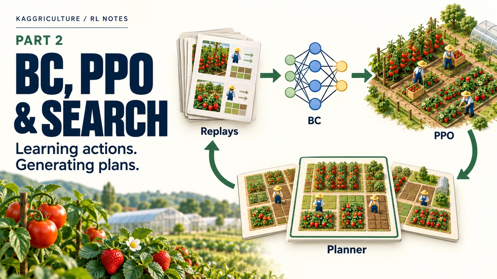
Having a strong strategy does not make the next improvement obvious. Hiring one more worker might waste money. Buying land can leave too few workers to maintain it. Planting more tomatoes can drive the price down just when the harvest arrives. Faster benchmarks do not create a new strategy when the program has no useful way to change its decisions.

An observation is the information the agent can currently see: cash, fields, workers, and markets. An action is a command such as hiring, moving, or selling. A policy is a function that maps an observation to an action. It can be written as rules or learned as a neural network.

Strong Kaggriculture entries improved this function in several ways. They learned the relationship between observations and actions from strong agents’ records, played new games with the resulting policy, and adjusted its action probabilities. They also used economic rules to search over workers, crops, and task schedules. These are behavior cloning, PPO, and plan search.

Method	What it changes	Learning or search signal
BC, Behavior Cloning	Neural-network weights mapping observations to actions	Probability assigned to a strong agent’s action
PPO, Proximal Policy Optimization	Weights of a stochastic policy that generates new experience	Outcomes that were better or worse than expected
Plan search	A plan combining workers, crops, tasks, movement, and trades	Feasibility and estimated revenue and costs

People designed the inputs, representations, and ways to make changes. Algorithms then adjusted many action probabilities and plan candidates within that design. The competitors did not inspect all 719 decisions in every game and edit each one by hand. Nor did the algorithms discover the entire farming economy without human design.

1. From replays to a policy on one RTX 5090

The 10th-place single-RTX-5090 writeup describes a relatively modest setup. The author trained BC on recent games from strong agents, then continued with PPO in a JAX environment, generating fresh experience in batches of 64 games. The reported times—about 3.5 hours for data preparation and BC, followed by about 19 hours of PPO—come from the author. The public code explains that the original BC checkpoint was lost and replaced by a retrained one. The historical training run and the published reproduction procedure are therefore not the same execution.

The code reference here is public commit 8aa3476. Its model takes the visible farm and market information and outputs worker tasks, targets, quantities, and market orders. It makes concrete decisions every turn rather than merely selecting one of a few prewritten strategies.

BC samples from 2,380 games

A teacher is the agent whose demonstrations BC learns to imitate. This dataset uses both seats from 2,380 games played by strong agents. Each seat makes 719 decisions per game:

\[2{,}380\times719\times2=3{,}422{,}440\]

Those 3.42 million samples are not 3.42 million independent games. They are successive observation–action pairs within games. The split contains 1,891 training games and 489 development games, with both seats of a game kept in the same split. Putting one seat in training and the other in validation would make the evaluation optimistic: the two seats share a market and random events.

The conversion centers on build_episode():

1. Create an environment using the original game’s configuration and seed.
2. Encode the observation available to each seat at that moment.
3. Convert the teacher action into the model’s action representation.
4. Advance the environment using the original actions from both seats.
5. Save samples with the relevant execution results, quantities, and targets.
6. Check that the final cash matches the original record.

For example, an input describing “the fifth day, 700 cash, four workers, and two shops creating tomato demand” might be paired with “hire another worker.” On the same day, a different cash balance and farm state might be paired with no hiring. BC can learn decisions conditioned on the current situation, rather than only memorizing a calendar.

The network does not receive the entire game JSON or the sentence “700 cash.” An encoder converts the observation into numerical arrays with a fixed ordering. In this implementation, map contains spatial farm information, global contains time and economic information, and unit_feat and unit_pos describe worker states and positions. The input contract specifies where each quantity goes and how it is scaled. Input-array and mask declarations

At the other end is a decoder. It selects from the model’s action probabilities and converts task types, targets, quantities, and market orders into commands accepted by the engine. Converting recorded commands into training labels must preserve the same meanings.

Boundary	What to check for one decision
Observation → numerical arrays	Which moment do the cash, position, and crop values describe, and where are they stored?
Teacher command → action label	How are the commodity, quantity, and task target represented as indices?
Model output → executable command	Does converting the same indices back into commands preserve the intended action?

An action mask marks choices that are unavailable. It can exclude tasks for nonexistent workers or commands that lack the necessary resources, leaving probabilities to be normalized over the remaining choices. If labels and masks disagree, the model may be unable to assign probability to the teacher’s action, or training and execution may solve different decision problems.

BC raises the probability of the demonstrated action

Suppose we reduce one decision to three actions. The teacher sold wheat, and the current model assigns these probabilities:

Action	Current model probability
Sell wheat	10%
Buy wheat	20%
Do not trade	70%

A loss measures how poorly the model matches its target. BC assigns a larger loss when the model gives the teacher’s action a lower probability. The basic expression is the negative logarithm of that action’s probability:

\[L_{\mathrm{BC}}=-\log \pi_\theta(a_{\mathrm{teacher}}\mid s)\]

Here, $s$ is the encoded observation, including the earlier 700 cash, four workers, fields, and shop information. The action $a$ is the teacher’s command in that situation, and $\theta$ denotes the network weights. The symbol $\log$ denotes the natural logarithm; exp is its inverse. A teacher-action probability of 1 gives a loss of 0, while a probability approaching 0 produces a large loss. Initially, $-\log0.1\approx2.30$. If learning later raises that action’s probability to 60%, the loss falls to $-\log0.6\approx0.51$.

Winning does not appear directly in this loss. It measures how little probability the model assigned to the teacher’s choice in the same observation. BC minimizes the average loss across samples. PPO instead learns from the consequences of the policy’s own choices.

Logits, gradients, and one update

A network need not directly output probabilities summing to 1. It can output an unrestricted real number—a logit $z_i$—for each action, then apply softmax. Exponentiation makes every $e^{z_i}$ positive. Dividing by their sum produces probabilities that add up to 1, with larger logits receiving more probability.

\[\begin{aligned} p_i&=\frac{e^{z_i}}{\sum_k e^{z_k}},\\ \frac{\partial L_{\mathrm{BC}}}{\partial z_i}&=p_i-y_i. \end{aligned}\]

The target $y_i$ is 1 for the teacher’s action and 0 elsewhere. Since the teacher chose the first action, the target vector is [1, 0, 0]. We can initialize the logits as log([0.1, 0.2, 0.7]); applying softmax recovers the original probabilities.

The gradient $\partial L/\partial z_i$ describes how the loss changes when a logit increases slightly. A gradient of −0.9 for selling means that raising the selling logit reduces the loss. It does not instruct us to add −0.9 to the probability. We change the logits first, then recompute probabilities through softmax.

Action	Target $y_i$	Current $p_i$	Gradient $p_i-y_i$	Logit change that reduces loss
Sell wheat	1	0.1	−0.9	Increase
Buy wheat	0	0.2	+0.2	Decrease
Do not trade	0	0.7	+0.7	Decrease more

Figure 2. One logit update with learning rate 0.5 in the three-action example. SELL probability rises from 0.100 to 0.189. BUY probability can rise from 0.200 to 0.218 even though its logit decreases, because all three probabilities are normalized together.

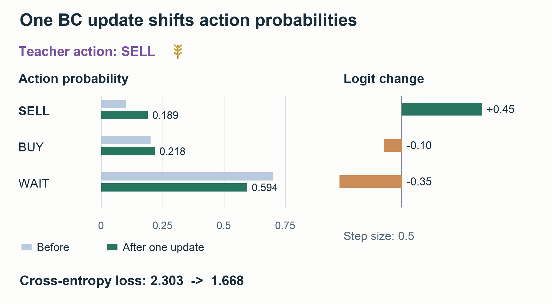
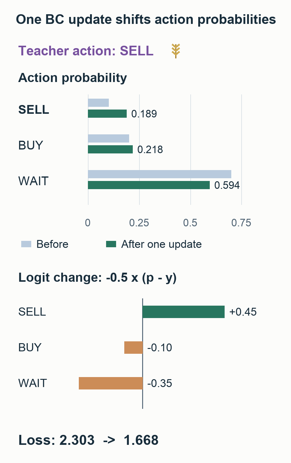
Gradient descent uses new value = old value − learning rate × gradient. One update with learning rate 0.5 requires only the Python standard library:

import math

def softmax(logits):
    peak = max(logits)
    weights = [math.exp(z - peak) for z in logits]
    return [w / sum(weights) for w in weights]

logits = [math.log(p) for p in [0.1, 0.2, 0.7]]
target, learning_rate = 0, 0.5
before = softmax(logits)
gradient = [p - (i == target) for i, p in enumerate(before)]
updated = [
    z - learning_rate * g for z, g in zip(logits, gradient)
]
after = softmax(updated)
print("before:", [round(p, 4) for p in before])
print("after: ", [round(p, 4) for p in after])
print("loss:  ", round(-math.log(after[target]), 4))

The output is before: [0.1, 0.2, 0.7], after: [0.1887, 0.2177, 0.5935], and loss: 1.6676. Selling probability has reached about 18.9%, not 60% in one step. The buying logit fell, but its probability rose slightly. Softmax normalizes each action relative to the others, so individual logit changes cannot be read as independent probability changes.

In the code, target = 0 identifies selling, the first action, as the target. The expression (i == target) becomes 1 at that position and 0 elsewhere, implementing $y_i$. Subtracting peak prevents overflow when exponentiating large numbers. Subtracting the same constant from every logit leaves the softmax probabilities unchanged.

This code changes the logits of one state directly. Real BC changes the network weights that produce those logits, propagating gradients backward through its layers. Other states sharing those weights change as well. That sharing enables learning and generalization, but it can also damage previously good behavior.

Backpropagation connects two effects: how a weight changes an output logit, and how that logit changes the loss. Differentiation rules compute each weight’s influence without requiring a person to perturb every weight and rerun the loss calculation.

The GPU is not individually playing “a program with hiring rule 1 changed” against “a program with selling rule 2 changed.” It processes many samples through the network to calculate gradients. An optimizer converts those gradients into weight updates. The example uses simple gradient descent; an optimizer such as Adam also uses information about recent gradient magnitudes and directions. The learning rate controls the scale of an update.

The actual BC implementation also has an auxiliary loss for predicting the opponent’s trades. Future trade records serve as training targets; the submitted agent is not given future trade answers as inputs. The training arguments are in repro/02_train_bc.sh.

From individual imitation to a complete farming policy

Teacher records contain connected behavior. Buying land is followed by states in which workers use the expanded farm. Planting tomatoes is followed by watering and harvesting. The model learns the next action at many points along these sequences.

It may fail to preserve the sequence. If the teacher hired a worker but the model did not, the model must subsequently operate a different farm from the one in the teacher’s record. This difference in states caused by the model’s own actions is an important weakness of BC. Matching teacher actions in recorded states and successfully running a farm for 30 days are separate tests.

BC’s immediate goal is a strong starting policy that passes both tests. Surpassing the teacher is a further objective.

2. How PPO changes an existing policy

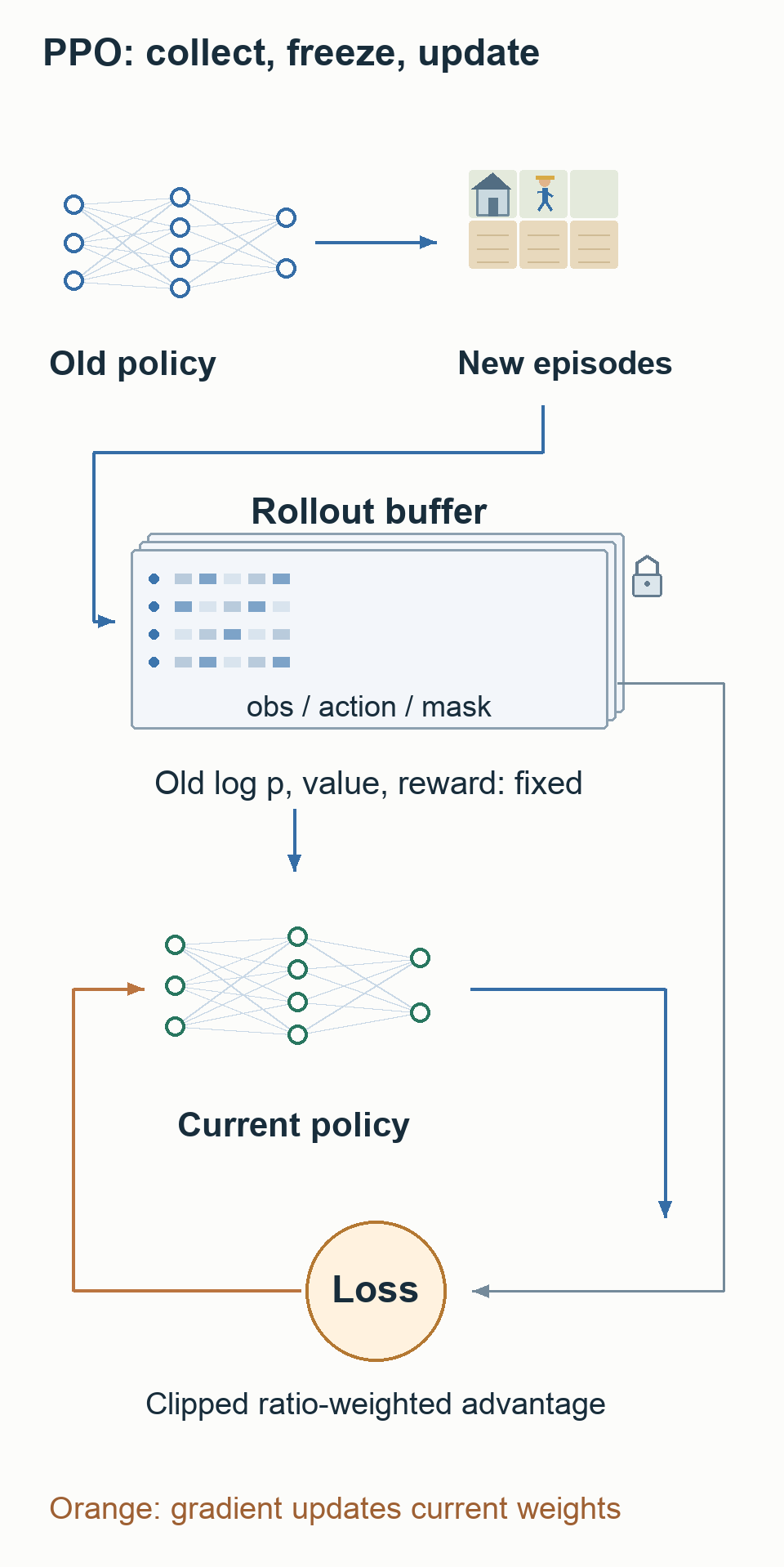
PPO uses the BC policy to play new games. Actions are sampled from the model’s probabilities. The same situation can therefore produce different commands, allowing the policy to experience departures from its usual behavior.

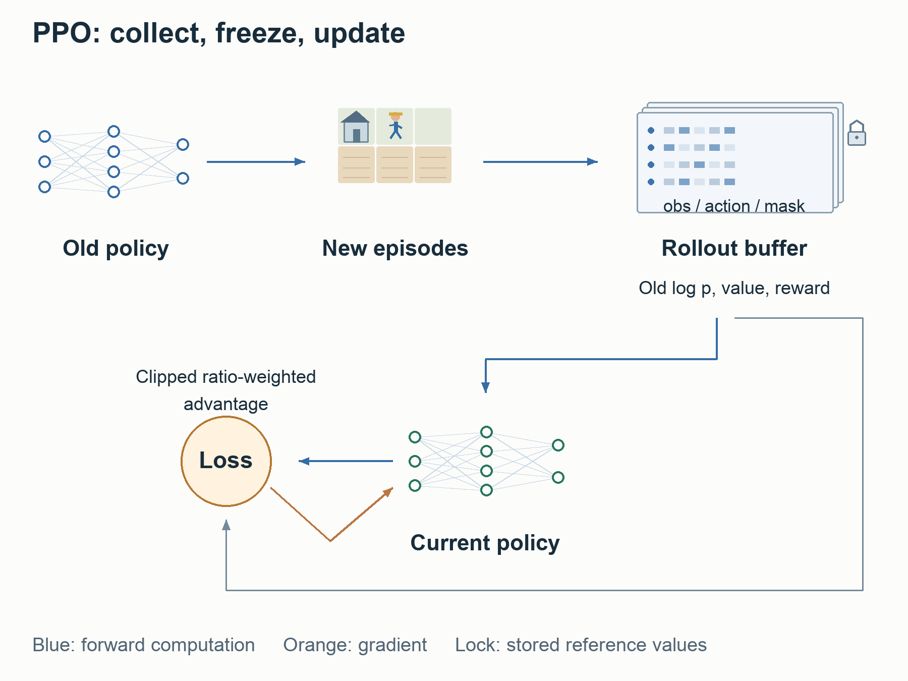
Saving only the final cash is insufficient. Training also needs to know what the policy saw, what it chose, the probability of that choice, and how good it expected the outcome to be.

A reward expresses a game outcome as a number for learning. A return is the sum of future rewards, potentially discounting rewards further in the future. The actor computes action probabilities. The critic predicts the expected return from the current observation; that prediction is the value. The critic does not directly decide whether to hire a worker. It supplies a baseline against which the actor’s outcome can be compared. The two outputs may share a neural-network backbone.

A rollout is the process and resulting sequence of data produced by playing with the current policy. PPO collects rollouts, then uses them to update the actor and critic.

Experience field	Meaning
Observation $s_t$	Cash, fields, workers, and markets at that turn
Chosen action $a_t$	The selected tasks, hiring commands, and market orders
old_logp	Log probability of that action under the policy that collected it
value	The critic’s return prediction at collection time
Reward	Game outcome expressed as a learning signal
Policy, opponent, and seed identifiers	Whose experience it is and which world produced it

A strong opponent’s public replay does not contain our policy’s old_logp. Rather than treating that record as fresh PPO experience from our current policy, we first use it for BC, then collect new experience with the learned policy.

When a turn contains multiple worker tasks and market orders, the action probability is the probability of choosing those commands jointly. Sequential conditional probabilities are multiplied; their log probabilities are added. The allowed choices affect that calculation, making the masks part of the probability definition.

Reward, value, and advantage

The final configuration of the single-5090 solution uses a terminal reward equal to the difference in final cash divided by 30,000 and clipped to −1 through 1. $M_{\mathrm{self}}$ and $M_{\mathrm{opp}}$ are our final cash and the opponent’s final cash. Their difference is the bank margin, measured in coins, not a difference in win points or Kaggle rating.

\[R=\operatorname{clip}\left(\frac{M_{\mathrm{self}}-M_{\mathrm{opp}}}{30{,}000},-1,1\right)\]

A 6,000-coin lead gives $+0.2$. Any lead of at least 30,000 coins gives $+1$. Unlike a reward based only on winning or losing, this reward assigns different values to wins of different sizes within the unclipped range. Whether increasing it also improves actual win points needs separate evaluation. The setting is in ppo_common.sh.

Suppose the critic predicted $+0.05$ from a farm state, but the eventual terminal reward was $+0.20$. The outcome was $+0.15$ better than expected. Advantage is a learning signal estimating how good a choice’s outcome was relative to that expectation. The critic’s value supplies the baseline.

Actual PPO connects rewards and next-state values through GAE. It does not simply attach the final reward to every action unchanged or declare every decision in a winning game correct.

Figure 3. Blue arrows carry data and forward computations through the network; orange arrows carry gradients back to the current weights. The lock marks collection-time log probabilities, values, and rewards that remain fixed. Advantages calculated from these records also remain fixed during the update.

Probability ratios control the update incentive

Suppose an action had probability 20% when the experience was collected and has probability 22% under the model being updated. The ratio is 1.1:

\[\begin{aligned} r_t(\theta)&=\frac{\pi_\theta(a_t\mid s_t)}{\pi_{\mathrm{old}}(a_t\mid s_t)},\\ \log r_t(\theta)&=\log\pi_\theta(a_t\mid s_t)\\ &\quad-\log\pi_{\mathrm{old}}(a_t\mid s_t). \end{aligned}\]

Implementations subtract log probabilities and apply exp to recover this ratio. PPO maximizes the following clipped objective for a sample. Here, the update hyperparameter is $\varepsilon=0.2$, giving a comparison interval of 0.8–1.2. Training code minimizes the negative of this objective.

For example, old_logp = log(0.20) is approximately −1.6094, and new_logp = log(0.22) is approximately −1.5141. Exponentiating their difference gives 1.1. This measures how much more or less likely the same action has become since collection. The $A_t$ in the next expression is the advantage already calculated for that experience.

\[\ell_t=\min\left(r_t A_t, \operatorname{clip}(r_t,0.8,1.2)A_t\right).\]

Clipping acts differently depending on the advantage’s sign. The table uses an old probability of 0.20. Increasing the probability of a positive-advantage action, or decreasing the probability of a negative-advantage action, should not improve the objective without limit. The direction comes from an estimated learning signal.

$A$	New probability	Ratio $r$	Original term $rA$	Clipped term	Minimum $\ell$
+1	0.22	1.1	+1.1	+1.1	+1.1
+1	0.30	1.5	+1.5	+1.2	+1.2
−1	0.10	0.5	−0.5	−0.8	−0.8
−1	0.30	1.5	−1.5	−1.2	−1.5

Figure 4. The horizontal axis is probability ratio $r$; the vertical axis is the sample's PPO objective $\ell_t$. Gray dashed lines show $rA$, and orange lines show the clipped objective. With $\varepsilon=0.2$, positive $A$ produces a flat region at $r>1.2$, and negative $A$ at $r<0.8$. The operation does not clip the reward itself.

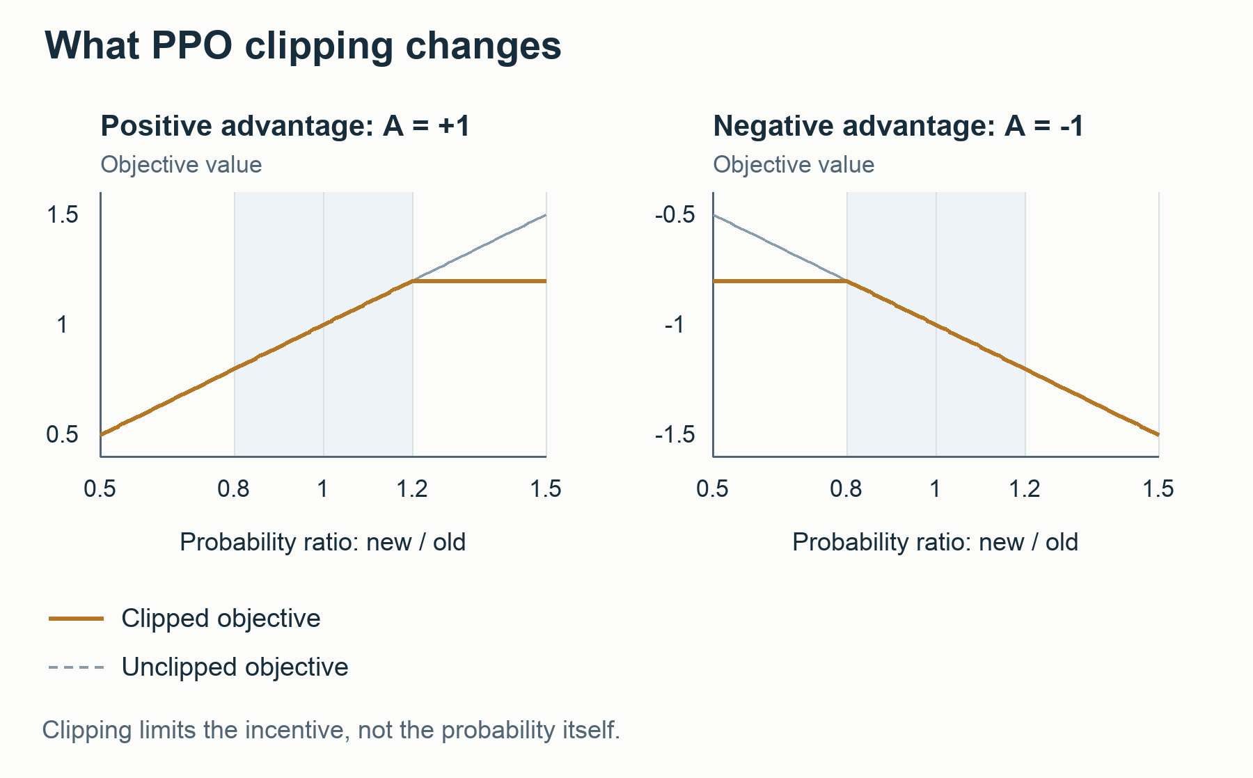
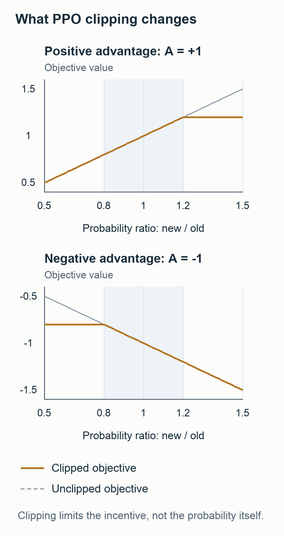
In the second row, raising the probability above 0.24 no longer increases this term. In the third, lowering it below 0.16 has the same saturation effect. In the fourth, increasing the probability of a negative-advantage action continues to worsen the objective.

def ppo_term(old_p, new_p, advantage, epsilon=0.2):
    ratio = new_p / old_p
    clipped = min(1 + epsilon, max(1 - epsilon, ratio))
    return min(ratio * advantage, clipped * advantage)

for advantage, new_p in [(1, .22), (1, .30), (-1, .10),
                         (-1, .30)]:
    term = ppo_term(.20, new_p, advantage)
    print(advantage, new_p, round(term, 2))

The final numbers are 1.1, 1.2, -0.8, -1.5. Clipping does not forcibly confine the probability to 0.16–0.24. Other samples sharing the network weights, or other loss terms, can move it beyond that interval. Implementations therefore also monitor KL divergence, a measure of distribution change, and may stop updates. Even a small average KL does not guarantee that a deployed policy choosing only its highest-probability action will preserve its behavior. The PPO paper and Spinning Up’s equations and explanation explain the clipping distinction. The 5090 implementation’s update is in ppo.py.

The old probabilities and advantages stay fixed

While training on one rollout, old_logp and advantages remain stored constants. The actor learns through new_logp calculated by the current policy; the critic learns through a separate value-prediction loss. If advantage changed along with the weights, the reference used to judge the action would move too. Automatic-differentiation code marks this boundary with stop_gradient or .detach(). An array computed earlier and stored in a buffer is already outside the differentiation path through the current weights.

Overwriting old_logp with the current policy’s probabilities would keep the ratio at 1. Mixing arbitrary experience from many old policies would instead violate PPO’s assumption that updates use the current collection distribution. The loop collects a fresh rollout, makes a limited number of updates on that batch, and then collects new experience. Spinning Up’s buffer and update implementation

This does not prove that one particular hire caused a win. Shop draws, opponent actions, and many other decisions contribute. A critic and many fresh experiences reduce noise and estimate a useful direction. BC matters especially in a game requiring long investment chains: random legal actions are unlikely to accidentally complete hiring → expansion → production → harvest → sale.

The single-5090 approach also did not assume that more PPO would automatically improve the policy. It used KL constraints toward the teacher distribution, a small learning rate, and distribution-change guards. Experience reuse and KL-based early stopping were controlled as well.

One cycle is freeze collection weights → collect a fresh rollout → calculate advantages from stored rewards and values → recompute current probabilities on the same observations → update weights. Computing PPO loss does not require playing another complete game for every proposed weight change. Games happen during collection; updates run the stored observations and actions through the network again.

3. The winners improved the teacher as well as the policy

The winning team also began with BC from strong agents’ records. Its final development path was broader than “BC once, then PPO forever,” as documented in training-lineage.md.

Figure 5. The winning team's original Training Loop diagram. Weaknesses involving tomato demand and shop conditions lead to heuristic-planner improvements and additional BC demonstrations for those conditions. Source: msdsm, kaggriculture-1st-solution.

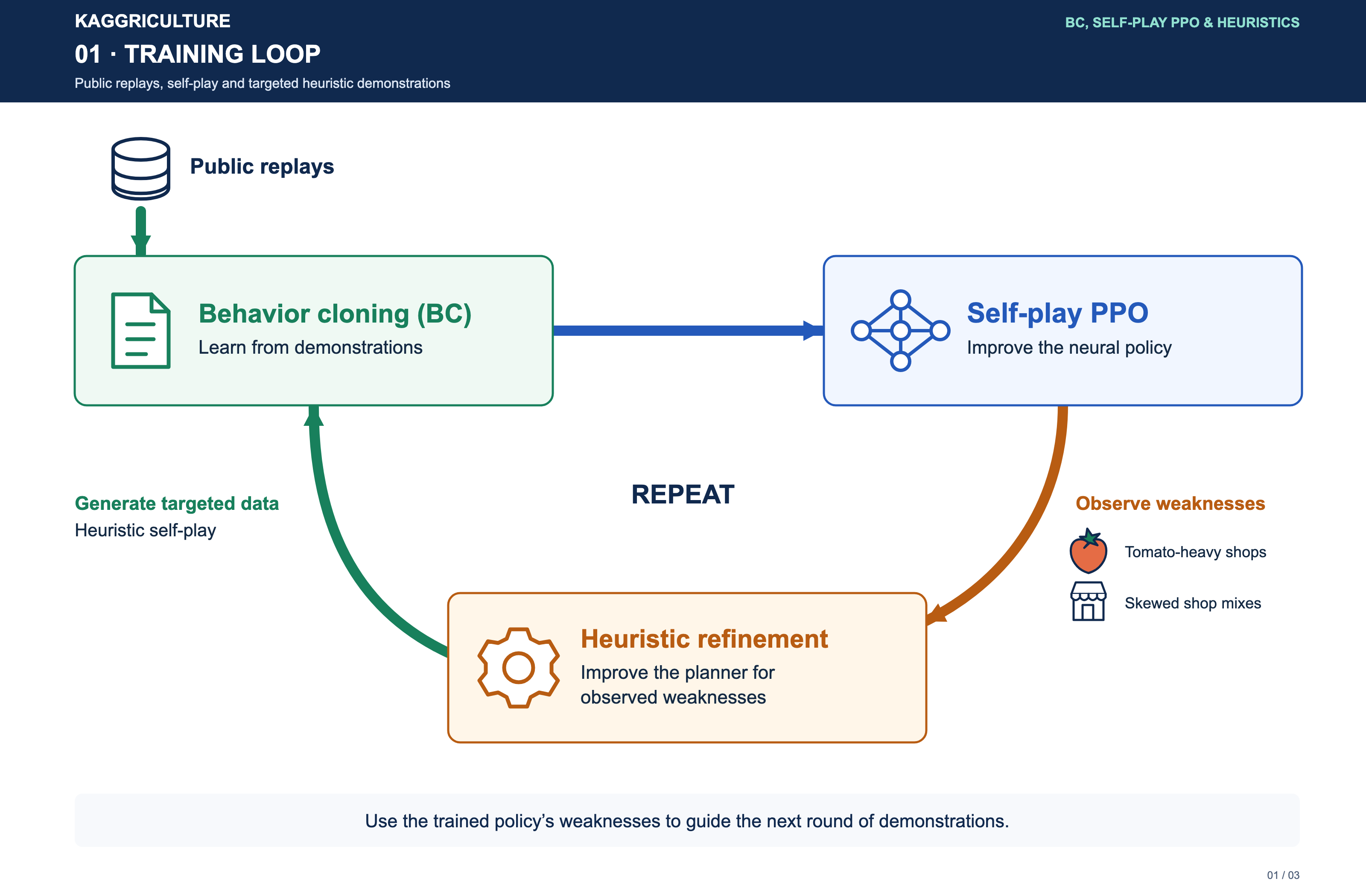
The learned policy was weak in worlds with high tomato demand or a concentration of particular shop types. The team improved a planner, a program that uses economic rules and search to construct an operating plan, and added complete games under those conditions to the BC data.

Running PPO longer relies on the current policy eventually attempting a good tomato strategy. Improving the teacher can put that strategy directly into the demonstrations. The planner supplies a long investment-and-work sequence that the policy may have difficulty discovering on its own.

How the winning code constructs BC samples

The winning repository is read at commit 84057a0f. prepare_replays.py produces these arrays for one teacher seat:

Array	Shape	Contents
features	719 × 264 × 124	Observation tokens and features at each decision
labels	719 × 30	Targets for up to 20 units and 10 market-order slots

This input format differs from the single-5090 implementation. Both encode observations and attach action labels, but their arrays are not interchangeable.

A token here is not a word. It is a position representing an entity such as a field tile or worker. Each position holds 124 numerical features. The shape 719 × 264 × 124 means that each of 719 decisions has 264 information positions, each represented by 124 numbers. The 30 label positions correspond to 20 unit actions and 10 ordered market slots. Nonexistent units and ignored targets are excluded from supervised action cross-entropy. Entropy and teacher KL still apply to real units and all ten market slots at those observations. Label and regularization handling

The 264 tokens cover 200 tiles across the two farms, up to 40 units, global state, commodities, estimated opponent inventory, market-order positions, and related information. Attention learns which other positions to consult when interpreting a position—for example, a worker’s nearby crops and relevant market demand. A Transformer repeats this operation through a network. Instead of receiving the opponent’s actual hidden inventory, the model uses estimates derived from changes in observations.

Alignment matters. An observation in steps[t] is paired with the action stored in steps[t+1], because the action is recorded on the row after execution. Shifting that pairing by one row breaks the question BC is meant to learn: what did the agent see before choosing this action?

Targets are not always raw command strings. Failed commands with no effect are excluded from action cross-entropy; selling labels use the quantities actually executed. Order is preserved. This does not mean every buy quantity is also replaced by the executed quantity: buy and sell labels are handled differently. label_actions() and legality handling make those distinctions explicit.

Critic warmup before PPO

BC teaches the model to match teacher actions. It does not automatically make a critic sharing that network accurate at predicting returns. A poor value baseline can push an otherwise competent policy in an unhelpful direction.

The published procedure freezes the actor and Transformer backbone, collects self-play data, and first trains only the critic that maps backbone outputs to values. The backbone is frozen, so its weights receive no gradients. Caching its output features also avoids rerunning its forward pass for each critic update. When saving the best checkpoint, the procedure checks that the actor’s hash is unchanged. PPO subsequently trains the backbone and actor again. critic.py

The winning repository’s default PPO reward differs from the single-5090 configuration. It uses the sign of the terminal cash difference: $+1$ for a win, $0$ for a draw, and $-1$ for a loss. A one-coin win receives the same reward as a large win. rollout.py

The published default GAE calculation has this form:

\[\begin{aligned} \delta_t&=R_t+\gamma V(s_{t+1})-V(s_t),\\ A_t&=\delta_t+\gamma\lambda A_{t+1}. \end{aligned}\]

Here, $R_t$ is the reward at that time, distinct from the earlier probability ratio $r_t$. The value $V(s_t)$ is the critic’s prediction from the visible cash, fields, workers, and markets. The quantity $\delta_t$ measures how much the previous expectation was off, using the reward received after one turn and the next value prediction.

The defaults are $\gamma=1$ and $\lambda=0.97$. The discount factor $\gamma$ controls future rewards; $\lambda$ controls how strongly errors from later steps propagate backward. At game termination, the next value and advantage are set to 0, and the calculation proceeds backward from the final turn. The quantity $\delta_t$ is the temporal-difference, or TD, error. The calculation uses the final outcome together with the critic’s intermediate estimates.

The critic’s target is return = advantage + value, using the value stored at collection time. This target array is not necessarily the same as summing every actual future reward: intermediate critic predictions can contribute.

Suppose a game contains only two decisions. The critic predicts 0.1 initially and 0.2 at the second decision, and the game ends with a winning reward of 1. Working backward gives:

Time	Reward $R$	Collected $V$	Next $V$	TD error $\delta$	Advantage $A$	Critic target $A+V$
Final $t=1$	1	0.2	0	0.8	0.8	1.0
Initial $t=0$	0	0.1	0.2	0.1	$0.1+0.97\times0.8=0.876$	0.976

At the final decision there is no subsequent state, so 1 − 0.2 = 0.8 is both the error and advantage. At the first decision, calculate 0 + 0.2 − 0.1 = 0.1, then add the later signal 0.97 × 0.8. This propagates information about the terminal outcome to earlier decisions; it does not establish that the first action alone caused the win.

The initial critic target is slightly below 1 because $\lambda=0.97$ retains a contribution from the next value prediction. Using other predictions to construct a learning target is called bootstrapping. With $\lambda=1$, both targets in this two-step example would equal the final reward of 1.

rewards, values = [0.0, 1.0], [0.1, 0.2]
gamma, lam = 1.0, 0.97
advantages = [0.0] * len(rewards)
next_value, next_advantage = 0.0, 0.0
for t in reversed(range(len(rewards))):
    delta = rewards[t] + gamma * next_value - values[t]
    advantage = delta + gamma * lam * next_advantage
    advantages[t] = advantage
    next_value, next_advantage = values[t], advantage
targets = [a + v for a, v in zip(advantages, values)]
mse = sum((v - y)**2 for v, y in zip(values, targets)) / 2
learning_rate = 0.1
predictions = [
    v - learning_rate * 2 * (v - y) / len(values)
    for v, y in zip(values, targets)
]
print("advantage:", [round(a, 3) for a in advantages])
print("target:   ", [round(y, 3) for y in targets])
print("value MSE:", round(mse, 6))
print("new value:", [round(v, 4) for v in predictions])

The output is advantage [0.876, 0.8], target [0.976, 1.0], and mean squared error 0.703688. A small gradient-descent step moves the predictions from [0.1, 0.2] toward their fixed targets, to [0.1876, 0.28]. As with the logits example, this code updates the predictions themselves. A real critic updates the network weights that produce them. From the same experience, the actor learns action probabilities using advantage, while the critic learns value predictions using the gap to its fixed targets.

The winning implementation uses Huber loss for values rather than this example’s MSE. Both reduce prediction error, but Huber loss does not penalize very large errors quadratically as MSE does. Policy training also normalizes advantages to adjust their mean and scale. Changing that numerical scale does not change the game’s reward definition. Actual GAE and return calculation

During training, stored observation batches pass through the current network to calculate current action probabilities and values together. The actor loss uses current probabilities, old probabilities, and fixed advantages. The critic loss compares current values with fixed targets. A weighted sum of these losses is differentiated by backpropagation, updating the output layers and shared backbone. The updated weights then generate the next rollout. This is how probability ratios and prediction errors affect the farm’s subsequent decisions.

The objective combines the PPO policy term, value-prediction error, KL to a fixed teacher, and action entropy. jax.value_and_grad and Adam update many weights together. In the public default loop, the teacher mainly serves as a reference distribution to preserve. That fixed KL reference is distinct from self-play, in which two copies of the current policy play each other. objectives.py

Entropy and teacher KL serve different purposes

Term	Compared distributions	Direction of pressure	If too strong
Entropy bonus	The current policy’s own action distribution	Avoid concentrating on one action too early	Unnecessary randomness can disrupt good actions
Teacher KL penalty	Fixed teacher versus current policy	Preserve the teacher’s action distribution	Escaping the teacher’s weaknesses becomes difficult
Old/new KL check	Collection policy versus current policy	Monitor large distribution changes within an update	Training may stop too early

For three actions, entropy is $H(p)=-\sum_i p_i\log p_i$. It is maximized at the uniform distribution [1/3, 1/3, 1/3], where it is approximately 1.099, and approaches 0 near [1, 0, 0]. High entropy does not identify a good strategy. It encourages broader exploration among possible actions.

With teacher distribution $q$, the winning code’s KL is $\sum_iq_i\log(q_i/p_i)$. If the teacher strongly favors selling, this penalty discourages the current policy from casually abandoning that action. Entropy looks only at the current distribution; teacher KL compares it with a specific reference distribution. Fixed-teacher KL calculation

KL measures a change across probability distributions, not just the difference for one action. It is 0 when the distributions agree. The actor’s final loss contains the PPO term encouraging actions with good outcomes, an entropy term discouraging premature concentration, and a KL term charging for departures from the teacher. Improving the PPO term alone therefore does not guarantee a better overall update or stronger play.

4. What people designed and what algorithms computed

Automated learning does not make experiment design automatic.

Human design or choice	Repeated algorithmic computation
Which teacher versions and games to use	BC sample losses and weight gradients
Observation, action, and legality representations	Action probabilities for each state
Reward, KL, entropy, and learning rate	Advantages from fresh experience and PPO updates
Diagnosis of weak world conditions	Candidate plans for a given world
Search operations coupling hiring and production	Comparisons of tasks, routes, and crop combinations
Approximate future-revenue and risk formulas	Approximate scores of modified plans
Opponents and validation procedure for selection	Game outcomes under matched conditions

People did not handwrite every action responsible for a high score. They did design representations and modification operators that let the algorithm propose useful changes. Our weakness was not simply too few benchmarks. We did not sufficiently connect a diagnosed weakness to a change in the process that generated strategies.

The public winning materials establish this structure, but do not provide a complete experiment diary or contribution table for every manual change. They cannot tell us how many rating points one particular heuristic produced.

5. A plan the search algorithm can modify

The winning C++ planner’s core structures appear in terminal_search.cpp. Their nesting is more useful initially than every individual field:

Plan: a candidate for today's farm operation
 ├─ Route: one farmer's or hired hand's work route
 │   ├─ Task: which tile to visit
 │   │   └─ Option: the bundle of work performed on that tile
 │   └─ Warehouse deliveries, start time, and night-delivery flag
 ├─ Whether land expansion is allowed
 ├─ Inventory to retain by commodity and when to sell
 └─ Mode for preparation orders, including hiring and purchases

This search changes today’s executable plan, not neural-network weights. It builds alternatives from the current observation and evaluates them subject to cash and time constraints. Tomorrow, it receives the changed farm’s observation and plans again.

A Task contains coordinates and several Option alternatives. A crop tile can offer choices such as leave it alone, water only, fertilize and water, water and harvest, or harvest and remove. An empty tile can offer alternatives for planting different crops.

An Option stores not only actions but also the resulting tile state, required seeds, feed and fertilizer, products, and information needed for future-value calculations. A Route contains an ordered sequence of (task index, option index) pairs. Adding a route can increase the workforce used that day.

This representation turns “add three tomato tiles and two workers” into a rearrangement of task options and routes, instead of a manual edit of 719 command strings. A separate executor converts the modified representation into engine commands.

6. Change workers, land, and crops together

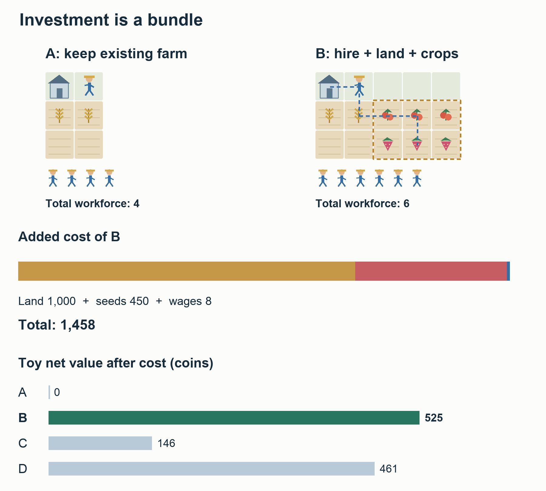
Consider a hypothetical state using the code’s cost rules. Days are zero-indexed, so day=4 means the fifth day. Initial hiring for that day is complete, giving four people including the farmer, with 4,000 coins in cash. The next land parcel costs 1,000 coins, and there are no seeds for the new crops. Existing farm-maintenance tasks still need to be done.

Candidate	Today’s total workforce	Expand land?	New tomato tiles	New strawberry tiles
A	4	No	0	0
B	6	Yes	3	3
C	6	Yes	6	0
D	6	Yes	0	6

A person need not enumerate this table by hand. The actual begin_search() creates initial plans with different workforce sizes and land-expansion settings. Later, full_search_step() removes and reinserts work, changes staffing by several people, and rebuilds the production mix. A code comment explains why: adding workers one at a time can cause search to reject an intermediate plan before reaching a profitable combination. Joint reconstruction operator

Hiring alone can lose money even when an expansion is valuable. Buying land alone can look poor even when a new production system is strong. Search needs to propose combinations that become profitable only when land, crops, and labor expand together.

Calculate B’s immediate spending

The code’s base wages rise with hiring order in a Fibonacci-like sequence. The cumulative hiring cost for a total workforce of four, including the farmer, is 4; for six it is 12. Since four are already present, adding two costs $12-4=8$.

Tomato seeds cost 50 coins and strawberry seeds cost 100. B’s additional spending is therefore:

\[\underbrace{8}_{\text{extra hiring}}+ \underbrace{1{,}000}_{\text{land}}+ \underbrace{3\times50}_{\text{tomatoes}}+ \underbrace{3\times100}_{\text{strawberries}} =1{,}458\]

C costs 1,308 and D costs 1,608. B immediately reduces cash by 1,458 relative to A. An evaluator maximizing only today’s balance would reject it.

Feasibility also requires spare operating cash. If the code calculates its reserve at the minimum of 75 in this state, $1{,}458+75\le4{,}000$ passes the cash check. The reserve is headroom used in a feasibility check, not an additional expense. Cash after spending is 2,542. Subtracting the reserve again from profit would double-count a cost. Hiring costs, evaluation, and reserve

Enough cash does not guarantee a feasible plan

B cannot assign work to new hands before they appear, plant seeds before they become available, or enter land before it opens. Neglecting existing harvests while tending the expansion can also invalidate the economics.

preparation_uncached_into() calculates hiring, land and seed orders together with availability times. A turn has at most 10 market orders. The calculation also accounts for when newly hired hands and purchased seeds become usable in the next farm-action phase.

The planner then coordinates each worker’s route and task schedule: where they start, how far they travel, when they plant, water and harvest, and whether they can return to the warehouse. A total workforce of six is insufficient by itself. The plan needs six Route objects that satisfy time and resource constraints.

7. Build future value from individual tiles

add_plant_variants() creates alternatives for crops that can be planted now. The code’s crop identifiers and timing rules include:

Crop	Commodity ID	Seed price	Age at first production	Later production interval
Tomato	2	50	8 days	1 day
Strawberry	3	100	10 days	2 days

Fertilizer, watering, and accumulated harvests affect later states, so value is not simply seed price times a fixed multiplier. enumerate() and value() enumerate work bundles for a tile and pass the resulting state to the next day.

A simplified tile-level comparison is:

\[\begin{aligned} V_{\mathrm{tile}}(x,d) &=\max_{o\in\mathcal O(x,d)}Q(x,d,o),\\ Q(x,d,o)&=\mathrm{immediate}(o)\\ &\quad-\mathrm{workCost}(o,d)\\ &\quad+\beta_d V_{\mathrm{tile}}(x',d+1),\\ x'&=\mathrm{next}(x,o). \end{aligned}\]

The state $x$ includes crop type, age, water, fertilizer, and remaining harvest capacity. The set $\mathcal O(x,d)$ contains the work bundles available that day. The quantity $Q$ scores one bundle. The calculation compares watering and waiting, harvesting, or removing a crop after its final harvest, including revenues and costs over the remaining days. When the same (tile state, day) appears again, the result is reused. This is dynamic programming, or DP.

This $V_{\mathrm{tile}}$ is different from the PPO critic. The critic is a neural-network prediction learned from experience; this function is calculated from human-written crop rules and cost formulas. Here $\beta_d$ discounts the next day’s calculated value. Sharing the letter $V$ does not mean the two calculations call the same model.

Suppose harvesting now earns 5, consumes work costing 1, and leaves no later revenue. Its value is 4. Waiting earns 0 today, costs 1 in work, and leads to a next-day value of 8. With $\beta_d=0.9$, its value is 0 − 1 + 0.9 × 8 = 6.2, so max chooses waiting. Tomorrow’s 8 comes from comparing the available choices in the same way. On the last day there is no future term, allowing values to be calculated backward. If multiple plans encounter the same tile state, the result can be retrieved from a cache.

Option.immediate is an intermediate score used to choose which work to place on a tile. The whole farm is evaluated separately. Adding tile-level estimated sales again after the market calculation would count the same revenue twice.

Convert work into dated production and costs

project_uncached() projects a tile’s future operation into three kinds of daily arrays:

q[day][commodity] : net changes in products and consumables
labour[day]      : later seed-purchase costs
work[day]        : approximate labor, including work and travel allowance

Despite its name, labour contains the cost of seeds bought later. Wages are calculated separately from work. Treating both arrays as labor costs would misread the economics.

Assume the example’s tomatoes and strawberries are watered daily, receive no fertilizer, and are harvested whenever production is available. Tomatoes planted on day=4 can be harvested on day=12, 13, 14, 15, and strawberries on day=14, 16, 18, 20. All these day numbers use the code’s zero-based indexing. With three tiles of each, the corresponding harvest dates yield three units. The actual DP also compares different watering, fertilizing, and harvest-timing options.

This stage records what is produced or consumed, in what quantity, and on which day for each tile. It does not yet determine the final revenue from three tomatoes. The full farm’s production must enter the market calculation; work must be converted to wages; and seed costs must be deducted before the plan’s future income and spending can be compared.

Future staffing is estimated anew each day

Kaggriculture’s hired hands disappear every night. The farm must hire the required workforce again the next day. This is not a model in which two workers hired today remain employed for the whole season. The reference engine clears hands=[] and resets hires_today=0 during night processing. Night processing

Future staffing is therefore estimated from each day’s expected work. The planner measures work in fifths of a turn and approximates one person’s effective capacity as 110 units, or 22 turns:

\[\widehat{n}_d=\max\left(1,\frac{\mathrm{work}[d]}{110}\right)\]

This headcount already includes the original farmer. Adding another farmer would overestimate wages. When staffing is fractional, the evaluator linearly interpolates between the cumulative wages for adjacent integer headcounts. For example, expected work of 385 gives 3.5 people. Interpolating between a wage cost of 2 for three people and 4 for four gives a cost of 3.

Today’s feasibility uses actual routes and actual hiring costs. Future comparisons use projected work and approximate wages so that many candidates can be evaluated quickly. Future labor costs

8. Production times current price is not future revenue

Producing 100 extra tomatoes does not necessarily earn 100 times the current tomato price. Selling increases market inventory and lowers the price. The opponent may sell the same commodity, while shops create demand in between. Production dates also differ.

The planner aggregates projected production across the farm, then advances market inventories by commodity and date. trade_difference() calculates the cash difference generated by predicted trades on both sides. The objective depends on our revenue and on how our supply changes the opponent’s sales revenue.

Suppose market inventory is 10,000 tomatoes and only we sell three units in sequence. Applying the code’s pricing and rounding yields sale prices of 60, 57, and 56, totaling 173—not the 180 obtained by pricing all three at 60. Larger volumes or simultaneous opponent supply make the distinction more important.

For today’s trades, goods must reach the warehouse before they can be sold. Revenue cannot be counted while a worker is still carrying the product at the far end of a field. market_timeline.inc extracts necessary PICKUP and DROP events from routes and processes warehouse capacity and market-order slots in sequence. Rather than recreating the entire world at every empty turn, it sparsely processes events that affect trading outcomes.

Unknown shops become demand scenarios

Future shop types are unknown. Opened shops are included directly; unrevealed shops are represented by multiple demand scenarios. Depending on how many shops have opened, the evaluator uses 32, 16, 8, or 1 scenarios. Once all shops are revealed, only one remains.

Future values across shop conditions are combined as follows:

\[F(p)=\operatorname{mean}_s F_s(p) -0.25\operatorname{std}_s F_s(p)\]

In this expression, $p$ is a plan and $s$ is a shop-scenario index. They are distinct from the earlier action probabilities $p_i$ and observations $s_t$. The value $F_s(p)$ scores future income and spending for plan $p$ under scenario $s$. The combined score subtracts one-quarter of the standard deviation across scenarios from their mean.

Each scenario accounts for daily demand, our production, and estimated opponent supply when calculating the cash difference, then deducts future seed costs and daily wages. A plan that works only under particular shop combinations is penalized for its variability. The coefficient 0.25 is a design choice for risk, not an official scoring rule. Combining future scenarios

Distant revenue is also discounted. From day=4, an amount received on day=12 is multiplied by $0.9^4\times0.97^4\approx0.58084$. The earlier 173 coins contribute about 100.49 to the evaluation. The actual sale still earns 173 coins. The discount is the planner’s way of giving less weight to distant, uncertain revenue when comparing it with immediate spending.

9. Compare the complete investment candidates

The whole-farm evaluator, evaluate_plan_summary(), follows this structure:

Reject infeasible preparation orders or schedules
Reject if purchases + operating reserve exceed current cash
Calculate today's routes, warehouse events, and trading cash difference
Add future value unless this is the final day
Deduct newly required seed and animal purchases

Conceptually:

\[J(p)=T_{\mathrm{today}}(p)+F(p)-C_{\mathrm{new\ inputs}}(p)\]

Today’s $T$ includes additional hiring and land costs and current-day trades. Future $F$ estimates subsequent production, market trades, hiring, and crop replacement. Current cash is common to all candidates and is not added. The quantity $J$ is a comparison score, not a direct prediction of the final cash balance. Nor are all the Option.value scores added to it; those values helped construct and prioritize candidates.

Tile-level work produces daily output and labor schedules. Scenario-specific market calculations turn these into $F$, which is combined with today’s trades and spending in $T$ to form $J$. The term $C_{\mathrm{new\ inputs}}$ is the cost of seeds and animals newly required today. The seed costs inside $F$ are for later crop replacement, so they do not deduct the same purchase twice.

Suppose A and B earn the same revenue from the existing farm today, differing only in the new investment and future value:

\[J(B)-J(A)=F(B)-F(A)-1{,}458\]

If $F(B)-F(A)$ is 1,700, B remains ahead by 242 after spending 1,458 today. If it is 1,300, B trails by 158. The comparison asks whether future proceeds, after accounting for the labor needed to maintain the new fields, exceed the additional spending now.

A small evaluator that chooses among four plans

Consider a toy evaluator with two accounting periods. Production, prices, and additional labor costs are specified for this example. Each tomato tile produces [3, 3]; each strawberry tile produces [0, 4]. Three price scenarios include high tomato prices with low strawberry prices and the reverse. The actual planner’s daily DP, price curve, and route checks are omitted.

Each plans entry is (workers, tomato tiles, strawberry tiles). The first prices scenario, ((100, 80), (70, 60)), means tomato prices of 100 and 80 across the two periods and strawberry prices of 70 and 60. In B’s first period, 3 tiles × 3 units = 9 tomatoes are produced and no strawberries. Net revenue before discounting is 9 × 100 − 2 × 6 = 888; after discounting it is 0.9 × 888 = 799.2. The inner loop performs this calculation for each period and scenario.

from statistics import mean, pstdev

plans = {"A": (4, 0, 0), "B": (6, 3, 3),
         "C": (6, 6, 0), "D": (6, 0, 6)}
prices = [((100, 80), (70, 60)),
          ((60, 50), (140, 120)),
          ((20, 20), (220, 180))]
discounts = [0.9, 0.81]

def evaluate(plan):
    workers, tomatoes, strawberries = plan
    plots = tomatoes + strawberries
    cost = {4: 4, 6: 12}[workers] - 4
    if plots:
        cost += 1000 + 50 * tomatoes + 100 * strawberries
    if cost + 75 > 4000:
        return float("-inf")
    q_tomato = [3 * tomatoes, 3 * tomatoes]
    q_strawberry = [0, 4 * strawberries]
    values = []
    for tomato_price, strawberry_price in prices:
        flows = []
        for d in range(2):
            income = q_tomato[d] * tomato_price[d]
            income += q_strawberry[d] * strawberry_price[d]
            future_labor = [2, 3][d] * plots
            flows.append(discounts[d] * (income - future_labor))
        values.append(sum(flows))
    future = mean(values) - 0.25 * pstdev(values)
    return future - cost

for name, plan in plans.items():
    print(name, round(evaluate(plan), 2))

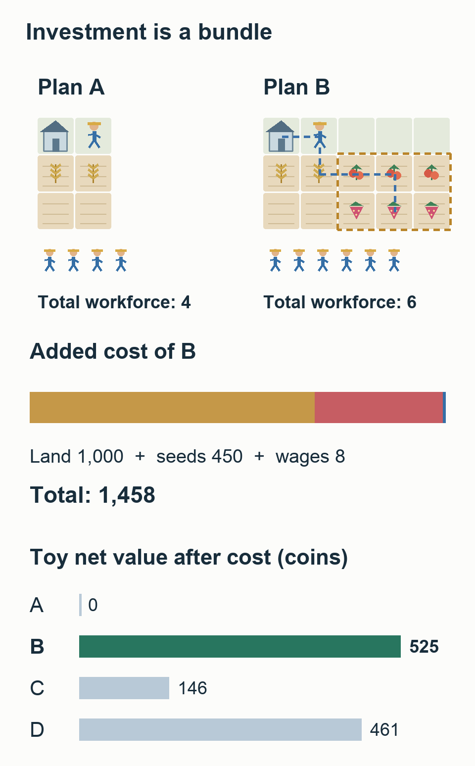
The evaluator returns 0 for A, about 525 for B, 146 for C, and 461 for D, selecting B. B’s scenario-specific future values are 1951.02, 1991.52, 2032.02. Their mean is about 1991.52 and standard deviation about 33.07. Subtracting a quarter of that deviation and today’s cost of 1,458 gives approximately 525.25. B is not the cheapest, but its mixed production leaves relatively consistent income across the three price conditions. Different prices or production would select a different candidate. The computation connects proposing candidates with evaluating them under the same objective.

Figure 6. Farm configurations and results from the toy evaluator. A retains existing operations; B expands the land and adds three tomato and three strawberry tiles. Total workforce includes the farmer. B's additional spending is 1,458 coins. The lower bars compare A, B, C, and D under the same objective. The fields and routes show the candidate configurations schematically.

The actual implementation aggregates production and consumption across tiles and updates q using the parts changed by a candidate modification. Work estimates produce daily wages. Prices respond to our supply and the opponent’s supply rather than remaining fixed. The toy omits those details but retains the structure of comparing plans by aggregating dated income and costs.

Which actual plan wins depends on the complete input: existing crops and their locations, revealed shops, inventory, opponent supply, and more. The calculation has not discovered a fixed rule that six people and three tomato tiles are optimal. It shows how to create feasible, connected alternatives for the current state and compare them with the same evaluator.

Fixed land costs can block useful search

A fixed cost creates a separate problem. If the first tomato tile on a new land parcel is charged the entire 1,000-coin land cost, it usually looks unprofitable. Rejecting that first tile prevents the second through sixth tiles from ever being considered.

During incremental task insertion, repair() temporarily adjusts for the new-land cost. It allows further tasks to be added instead of abandoning expansion because the first crop cannot pay for the entire parcel. The completed plan’s score still includes the land cost. This is not free land; it is a way to avoid rejecting an unfinished plan prematurely. Task insertion using the whole-farm score

Candidate generation needs a way to complete promising partial plans. Accurately scoring only fully constructed strategies does not solve that problem.

10. Incremental search and cached evaluation

The plan-search loop can be summarized as:

best = best initial plan across workforce, land, and inventory settings
current = best

while search time remains:
    proposal = modify tasks, routes, production, or staffing in current
    proposal = reconstruct under cash, time, and resource constraints
    score = lightweight events for today + estimated future value

    if better, or accepted despite a loss under the temperature schedule:
        current = proposal
    if proposal is better than best:
        best = proposal

return executable commands for today's best plan

Actual modifications include adding or removing tasks, replacing task options, reassigning work, changing visit order, rebuilding groups of production tiles, and changing workforce size. Simulated annealing sometimes accepts worse intermediate plans. Its temperature controls how much deterioration is tolerated. Good candidates are stored separately, and starting points from several production families are retained. These mechanisms reduce the chance of getting stuck after small improvements around one plan. search_methods.inc

The computation reuses results according to the structure of the problem:

Reuse or approximation	Computation avoided
Cache DP results for identical tile states	Recalculating remaining production and costs under the same conditions
Store dated tile production and modification deltas	Recomputing every tile’s future for each candidate
Apply only changed production and work	Recalculating unchanged parts of the farm
Cache commodity-specific scenario paths	Repeating market calculations for identical supply flows
Process warehouse arrivals and departures as events	Playing an official 30-day game for each candidate
Reuse route length and resource summaries	Expanding every route after a small edit

If one strawberry tile’s harvest date changes, the evaluator subtracts its previous production schedule from the totals and adds the new schedule. It calculates how that difference changes staffing and estimated sales. It need not simulate the entire farm from scratch.

Price forecasts also change. continuation_prices() calculates how one additional unit on a particular date changes the expected cash difference between us and the opponent. It mixes that marginal value 50:50 with the previous price forecast, then chooses tile-level work again under the revised prices. This can correct a plan that keeps valuing an overproduced crop as though every additional unit sold at the same price. Marginal production value and task replanning

The future model does not plan every investment across the remaining 30-day season. Starting from the farm produced by today’s investment, it estimates maintenance, harvests, and some crop replacement. It does not assume arbitrary new tomato and strawberry investments on all empty tiles tomorrow. The planner receives the actual observation at the next dawn and plans again. It models today’s executable work in detail and uses fast approximations for what follows.

11. Internal scores and independent match validation

Search must score many plans. Playing a complete game in the official engine for every candidate would severely limit the number it could consider. That is why it uses a less expensive internal evaluator.

If the evaluator’s assumptions are wrong, search chooses the wrong plan. Underestimating future labor costs or mispredicting opponent supply can make a losing plan look attractive. Complete games are still needed to establish whether an apparently good plan produces stronger play.

Both stages are necessary:

1. Candidate generation: use inexpensive approximations to compare many plans and construct connected alternatives.
2. Policy validation: play complete games under the real rules against separate opponents and worlds.

The winners’ public evaluation tool uses official engine 1.32.7 and swaps seats for the same seed. It does not reconstruct the competition’s entire opponent distribution or every historical promotion criterion. The important distinction is between an internal generation score and an external validation result. evaluate.py

PPO has an analogous limitation. When identical policies play each other and both seats are counted, the average win-point score is 0.5 when draws receive half a point. One side’s gain is the other’s loss. That number alone cannot show whether the next policy generation is stronger. Lower training loss, higher teacher agreement, higher search scores, and better results against independent opponents answer different questions.

12. Turn better plans into new demonstrations

The winners’ final BC data combined 849 seat trajectories from strong public agents with 600 planner-generated seat trajectories. Those 600 came from both seats of 300 planner games, not only from the winning sides.

Shop conditions used for demonstrations	Games	Intended coverage
Normal shop draws	100	Retain general farming behavior
At least two tomato-related shops	100	Weaknesses in high-tomato-demand worlds
At least three shops of the same type	100	Weaknesses when demand concentrates on one product

The data generator made underrepresented conditions more frequent. It changed the revealed shop types while retaining the normal reveal timing, rather than showing the policy future information early. Results in this deliberately modified distribution are not estimates of performance under the ordinary competition distribution. shop_scenarios.py

Retraining BC on planner-generated observation–action pairs teaches the network to reproduce those operations in similar situations. Subsequent PPO adjusts action probabilities using outcomes in states that the policy actually reaches while playing.

The pieces contribute different abilities. Search uses a human-designed economic model to produce strong demonstrations in particular worlds. The network generalizes across demonstrations and executes quickly. PPO changes that function using outcomes from its own experience. No single component supplies every function of the others.

13. Training-time search and submitted inference are different

The winning repository contains both a C++ search teacher that operates for a complete season and the final-day search used by submitted Agent A.

For teacher generation, the search policy operates from day 0 through day 29, making and executing a new daily plan from each observation. Final Agent A instead normally uses its neural network, handing control to the search controller on day=29, the final day. It preloads the library one day earlier and falls back to the network if too little overage time remains when search starts or if the handoff fails. SearchHandoff

The early investment and midseason production demonstrations therefore did not come solely from optimizing final-day harvesting: the teacher used search across the whole season. Nor did final Agent A run that large C++ search every day during submission play.

Agent B adds another execution improvement. Earlier choices’ resource consumption changes later workers’ masks, preventing multiple workers from consuming the same seed or duplicating work on one tile. These sequential constraints must agree across rollout collection, probability recomputation, and submitted inference. If sampling and training use different distributions, the PPO ratio is already wrong. Sequential action selection

Suppose there is one seed and two workers on different empty tiles, each choosing between plant/wait. The first worker’s probabilities are 0.6/0.4; the second’s before masking are 0.8/0.2. If the first plants, the second’s plant action is masked and its remaining wait action is renormalized to probability 1.

First worker	Seeds left	Second worker’s conditional probabilities	Joint probability
Plant	0	Plant 0, wait 1	Plant–wait $0.6\times1=0.6$
Wait	1	Plant 0.8, wait 0.2	Wait–plant $0.4\times0.8=0.32$
Wait	1	Plant 0.8, wait 0.2	Wait–wait $0.4\times0.2=0.08$

These three probabilities sum to 1. Independent sampling without the mask would assign $0.6\times0.8=0.48$ to the impossible outcome in which both workers plant.

For the first row, PPO should store log(0.6) + log(1). If training forgets the second worker’s mask and computes log(0.6) + log(0.2), the new/old probability ratio becomes 0.2 instead of 1 even though no weights changed. Matching the executed commands alone is insufficient. The sampled action, effective mask, stored probability, and training-time recomputed probability must describe the same distribution. This consistency does not require rerunning the backbone for each worker. The code calculates logits once, then sequentially restricts the valid actions according to earlier choices.

Conflicting or failed commands can erase a learned improvement. The strategy being learned and the faithful execution of its choices both matter.

14. Expanding the decisions our program could change

We also tried to modify existing strategies, found small improvements in records, and implemented learning to select more favorable alternatives. We did not lack the idea of changing the strategy. The changes our programs could attempt were narrow, and the strategy generators that might expand that range were not sufficiently connected to learning.

A model selecting prewritten routes can learn which route to use. It cannot invent early investments or task arrangements absent from those routes. A rule that changes one fertilizer or seed-purchase decision can improve that situation, but it does not jointly replan workers, land, and crop transitions.

A BC–PPO model can change actions every turn, while a planner can change staffing and task composition together. Rather than asking which algorithm is universally superior, ask which decisions must change to address the present failure, and whether the model can change them.

If the next competition exposes weak tomato farming, distinguish these cases before enlarging the model or renting more GPUs:

• Good tomato strategies already exist, but the program does not select them: investigate selection.
• The teacher farms well, but the BC policy’s tasks or orders fail: investigate representation, learning, and execution.
• The policy collapses in states outside the demonstrations after playing its own actions: investigate data coverage and fresh rollouts.
• Neither the candidate set nor the teachers contain a good strategy: investigate new teachers, search, or another strategy generator.

Each calls for different computation. A better selector can solve the first problem without creating the missing options in the fourth. A good planner for the fourth does not automatically fix execution errors.

15. Compute allocation for BC, PPO, and search

The single-5090 solution moved the environment into JAX and advanced multiple worlds on the GPU. The winners’ public pipeline connects Rust batch environments with JAX policy inference and learning. Their C++ plan search runs on CPUs. The parallelizable computation is identified before the hardware is chosen.

BC computes teacher-action probabilities and gradients across many observations. PPO executes the policy in many worlds to collect experience, then computes gradients from that experience. The planner evaluates estimated income and costs for candidates represented as tasks and routes. Complete-game benchmarks test whether the resulting policies are actually stronger.

According to the authors’ records, the retained ancestry of winning Agent A contains approximately 8.29 million PPO games. This is not the total workload including discarded experiments, teacher generation, critic fitting, and evaluation. It cannot be presented as having the cost of the single-5090 example. Conversely, that single-GPU result also contradicts the claim that trying BC → PPO requires the winners’ hardware scale. The practical requirement is to validate a complete improvement loop within the available resources.

Start with a small connected process. Convert one teacher game into observation–action samples and check that a small BC policy can operate the farm to completion. Collect a rollout containing action probabilities and values, then inspect how one PPO update changes actual choices. If new behavior is needed, first check whether the planner can represent and modify that plan. Raise throughput after the process works.

A benchmark compares candidates. Stronger candidates come from learning a policy from strong demonstrations, improving it with its own rollouts, or searching for a new operating plan. The next computation depends on what the program is capable of changing.

---

← Part 1: From Benchmarks to Strategy · Part 3: A Workflow Connecting Logs, Evaluation, and GPU Compute →