Kaggriculture RL, Part 3: A Workflow from Game Logs to Stronger Policies

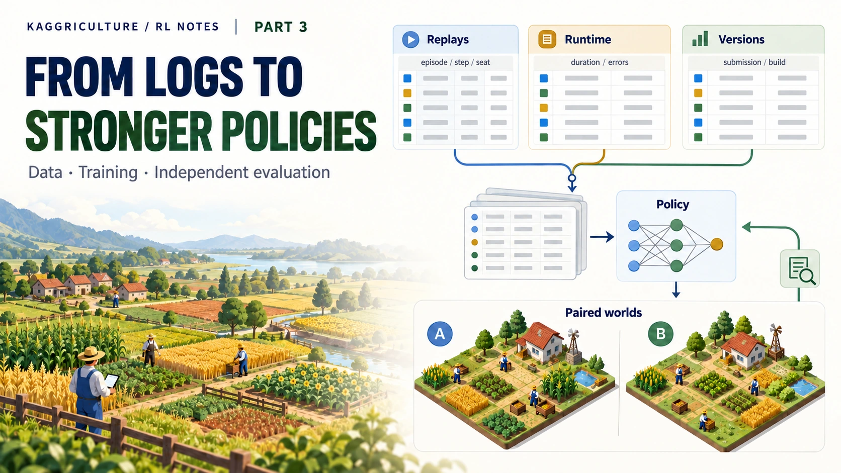
If you have rented a GPU but cannot say what computation to run, there is a question to answer before choosing the hardware: what inputs will produce new behavior, and what evidence will tell you that behavior is better?

I ran many matches during Kaggriculture. I inspected logs, developed small rules, and tried controllers that learned the value of choosing among existing alternatives. The weakness in that process was not simply a shortage of compute. Learning from strong play, generating strategies outside the existing menu, and testing against a changing field were not sufficiently connected.

BC needs observations, the information available at the time, paired with the teacher’s chosen actions. PPO needs new experience collected by running the current policy, the program that chooses actions. That experience is a rollout. A final decision needs match results that were not used for training. All three come from games, but serve different purposes. Deciding what to learn and what to verify determines which logs to collect and which computation to run.

The next competition needs a connected process: collect data → select teachers → generate and train policies → diagnose failures → evaluate independently. A failure should lead to better teachers or training examples, or to a change in the method that generates new play.

This is the workflow I would use in the next competition. The winning team’s public code connects BC, self-play, and teacher improvement, but does not prescribe every competition’s collection, evaluation, and release process. The implementation must fit the environment and the objective.

1. Choose the join keys before collecting logs

Each source answers a different question

Source	Main question	What it can change
Official full-game replays	How do the currently strong programs operate?	Teachers, production strategies, training conditions
Replays of my submissions	Where does my policy diverge when it meets real opponents?	Bug fixes, recovery data, training for specific weaknesses
Agent execution logs	Which branch ran, what failed, and where was the time spent?	Execution code and diagnostics
Submission metadata and leaderboard records	Which version produced this result, and when?	Teacher selection, opponent weights, interpretation of strategy changes
Training rollouts collected directly	How did my choices turn out relative to expectations?	The next PPO weight update

The full archive can reveal a strong operating strategy, while my own games show why I cannot execute it. Suppose an execution log says a purchase was canceled for lack of resources. First check whether the money was actually missing. If enough cash was available, fix the execution code. If an earlier investment really consumed it, investigate the investment sequence. If execution is correct but every available strategy loses under the same conditions, a different teacher or a new planning method is needed.

The execution logs I downloaded had empty stdout and stderr, so call duration was the main directly usable information. That does not mean execution logs can only tell us about runtime. My own agent can record which rule it selected, how post-processing changed the model’s command, and why a command was canceled. Being unable to inspect an opponent’s internal logs is different from leaving no explanation in my own program.

There is no need to print the entire observation every turn. Reuse information already present in the replay, and log the decision reasons that the replay cannot reveal. One example is considered buying land, but canceled to preserve cash for tomorrow's hiring. If output volume and runtime are limited, record important events and per-rule activation counts.

Joining on team names mixes different programs

A high team score today does not make that team’s week-old submission a strong teacher. The same team name can cover versions with different opening investments, products, and trading rules. Join on keys identifying the same game, seat, and program, rather than on names.

Game: episode_id, creation time, engine version
Seat: episode_id, seat, submission_id, team_id
Program: submission_id, publication/submission time,
         code hash or extent of identity verification
Rating: submission_id or team_id, observation time,
        whether the rating belongs to a submission or team
Execution: episode_id, seat, step, duration, internal events

If an API provides a team rating, do not relabel it as a particular submission’s rating. Mark intervals in which two versions from one team may be mixed around a replacement. Leave an unverified version unknown. That allows it to be excluded from teacher selection, or lets you check whether the conclusion survives without it.

Teacher selection also has a time boundary. If the question is how would selection using information available at the time have performed?, selecting historical records by post-competition scores introduces future information. BC that learns retrospectively from the best model after the competition has a different purpose. Decide which question the data is meant to answer.

Keep original files separate from a manifest: a list identifying the game, seat, version, and intended use of each example. Compare original hashes after moving files to confirm that their contents have not changed.

{
  "episode_id": 123456,
  "seat": 0,
  "submission_id": 765432,
  "engine_version": "pinned-engine",
  "replay_sha256": "...",
  "teacher_family": "early-expansion",
  "split": "train",
  "selection_as_of": "2026-10-01T00:00:00Z"
}

This format is an example for a future project. The winning team’s public package likewise takes an index that explicitly names teacher seats. It does not infer the teacher automatically from the winner or leaderboard rank. Teacher manifests, deduplication, and splits

Join five seat records

Consider five fictional game-seat rows, three execution-log rows already summarized by seat, and three submission-metadata rows. A seat is player position 0 or 1 in a game. There are 11 input rows in total, but the desired output has one row per game-seat, so it has five rows. A left join retains every base game-seat row and attaches matching information. Opponent seats do not disappear just because my agent has no execution log for them.

Raw execution logs usually have a row for each (game, seat, step), giving hundreds of rows per game. Summarize first-call duration, maximum call duration, and error counts by seat before making this one-row-per-seat join. To investigate a particular failed move, join to the replay on step as well. Attaching raw logs and then calculating win rate from hundreds of duplicated seat rows would count the same result repeatedly.

Game	Seat	Submission	Own bank / opponent bank	Match score	My execution log
101	0	10	100 / 80	1	Present
101	1	20	80 / 100	0	Absent
102	0	10	90 / 90	0.5	Present
102	1	30	90 / 90	0.5	Absent
103	0	10	70 / 85	0	Present

The following code uses only the Python 3 standard library. Money in rows is the recorded outcome; logs contains only each seat’s maximum call duration. The ratings in meta are team ratings observed at one time. They are not intrinsic ratings of submissions 10, 20, and 30.

engine = "toy-engine"
rows = [
    (101, 0, 10, 100, 80),
    (101, 1, 20, 80, 100),
    (102, 0, 10, 90, 90),
    (102, 1, 30, 90, 90),
    (103, 0, 10, 70, 85),
]

# Key: engine, episode, seat, submission.
logs = {
    (engine, 101, 0, 10): {"max_duration": 0.01},
    (engine, 102, 0, 10): {"max_duration": 0.02},
    (engine, 103, 0, 10): {"max_duration": 0.03},
}
snapshot_time = "2026-10-01T12:00:00Z"
meta = {
    10: {"team": "A", "team_rating": 2800},
    20: {"team": "B", "team_rating": 2500},
    30: {"team": "C", "team_rating": 2900},
}

joined = []
seen = set()
seen_seats = set()
for episode, seat, submission, bank, other in rows:
    seat_key = (engine, episode, seat)
    assert seat_key not in seen_seats
    seen_seats.add(seat_key)
    key = (engine, episode, seat, submission)
    assert key not in seen
    seen.add(key)
    point = 1.0 if bank > other else 0.0
    if bank == other:
        point = 0.5
    joined.append({
        "key": key,
        "point": point,
        "execution": logs.get(key),
        "team_snapshot": meta.get(submission),
        "snapshot_time": snapshot_time,
    })

assert not (set(logs) - seen)
mine = [r for r in joined if r["key"][3] == 10]
matched = sum(r["execution"] is not None for r in joined)
points = sum(r["point"] for r in mine)
print("inputs:", len(rows), len(logs), len(meta))
print("joined / logs / missing:", len(joined), matched,
      len(joined) - matched)
print("submission 10:", points, "/", len(mine),
      "=", points / len(mine))

The output is inputs: 5 3 3, joined / logs / missing: 5 3 2, and submission 10: 1.5 / 3 = 0.5. The original 11 rows are not 11 games, and the five joined seats are not five games of one policy. Submission 10’s denominator is three.

The scores of the two seats in one game are related. Joining the data establishes who did what and when; judging strength comes afterward. A single stored team-rating snapshot also cannot reconstruct the rating at the time of a game. To study change over time, save the timestamp whenever a rating is checked.

logs.get(key) and meta.get(submission) leave None when no matching information exists. My execution log being absent for an opponent seat is expected. A missing log for my own seat, or an unknown teacher version, means collection is incomplete. Count those reasons separately. Recording all seats → seats with verified versions → replays downloaded → own execution logs downloaded reveals which analyses lack input data.

Check duplicates before joining. In this example, seen and seen_seats prevent counting a game-seat twice. Python dictionaries such as logs and meta overwrite earlier values when a key is repeated. Check for conflicting records before converting CSV or JSONL inputs to dictionaries. Include time in the key for real time-series metadata, and do not attach a later score as though it had been known earlier.

2. A strong replay is not automatically a good teacher

Select coherent play, not just winning moments

Collecting only a strong player’s wins can omit recovery under unfavorable conditions. Mixing every highly ranked team can instead create conflicting opening plans. If one teacher invests in labor first while another saves cash for livestock, a mixture of their intermediate actions may complete neither strategy.

Start with one or a few strong, coherent versions to make problems easier to diagnose. Check whether the model matches actions on the teacher’s observations, and whether it can finish a game when played directly. Then add teachers for missing strategies. One model can learn multiple styles when observations contain enough information to distinguish them. The question is whether indistinguishable situations are being given conflicting targets.

The 70th-place replay BC and teacher-selection writeup describes starting broadly and then narrowing to strong, compatible teacher families. Teacher reputation and dataset size matter less than whether the representation and execution code can learn the complete operating strategy.

Check observation–action alignment one move at a time

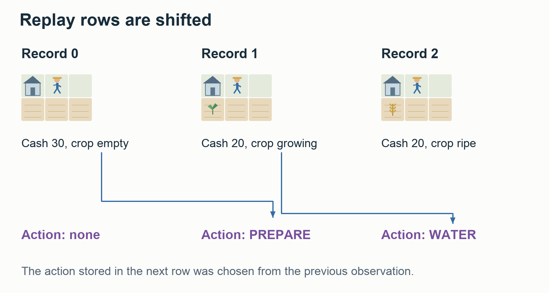
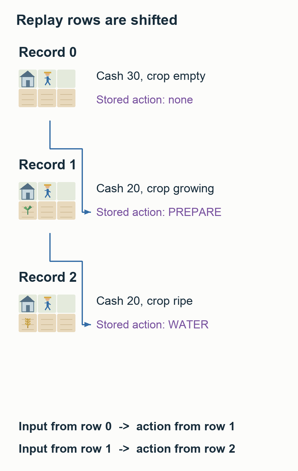
Find out whether the action in replay steps[t] was selected from observation[t], or was recorded as the result of an earlier observation. An offset of one row can make the model see an action’s consequences instead of the information that caused it.

The winning Kaggriculture extractor pairs observation[t] with action[t+1], producing 719 decisions from 720 states. That is not a universal instruction to shift every game’s labels by one row. Check the official recording convention and manually follow a few purchases, movements, or harvests with visible state changes. The extraction loop

Figure 7. Record alignment in the small farm example. In the winning extractor, the action selected from observation $t$ is stored in the next row, $t+1$. Row 0's empty field therefore pairs with PREPARE in row 1. Check each engine's recording convention rather than assuming other games use this format.

Expand a sample into five fields to make errors easier to find.

1. The observation seen immediately before the decision
2. The requested action and ordered market commands
3. What the engine actually executed, including failures
4. Labels retained for learning and labels ignored
5. The result of decoding the labels back into commands

If the 3 → 4 → 5 round trip is wrong, perfect imitation of the labels can still produce a weak farm. Overall accuracy can hide this. Matching movement and PASS while missing a rare hiring order can change hundreds of subsequent production decisions.

Preserve order positions and executed quantities

Suppose the player has 100 cash, sells goods for 50 in an earlier order, and makes an investment costing 120 in a later order. Sorting orders by type and executing the purchase first makes it fail for insufficient cash. Sorting for comparison has changed the policy.

Invalid orders cannot always be deleted when constructing labels. If the engine interleaves both players’ orders by slot, deleting slot 2 and moving order 3 forward changes its timing relative to the opponent. Decide whether to leave a SKIP in place, exclude that label from the loss, and distinguish requested from executed quantities. The decoder, which converts model outputs into actual commands, must follow the same conventions.

The winning code excludes labels for ineffective or unexecuted actions. For SELL, it labels the absolute quantity actually executed rather than the requested amount. It does not apply that same conversion to every purchase action. Different action types have different meanings even within one preprocessing pipeline. Label construction

The decoder must also account for resources consumed by earlier choices. Letting another worker use an already-spent seed, or treating goods in a worker’s bag as shed stock, can make the combined action fail even when individual predictions look correct. Goods dropped into the shed in the same turn can be sold during market processing, so restricting sales to the shed’s current contents is also wrong. Label construction, the mask of available choices, resource accounting, and actual commands must agree. The 24th-place execution and decoder analysis

Outcomes can be targets without becoming inputs

Learning the value of a current action from future rewards is fundamental to RL. Giving the policy a future shop it has not seen, or the opponent’s private inventory, is a different matter. Even if a spectator replay contains complete information, encode only the observations allowed to the player.

Some designs give the value function additional information during training, but explicitly separate that information from the acting policy. A small first pipeline is easier to inspect when input restrictions are consistent throughout.

3. Separate four uses of data

Splitting a dataset into train and validation does not complete competition evaluation. BC validation measures how well the model matches teacher actions on records it did not train on. Establishing that a policy plays more strongly requires actual matches. Four roles help distinguish those questions.

Role	Use	Can it be examined repeatedly?
Training	BC, value-function, and PPO updates	Within the update algorithm’s permitted use
Development	Representation, reward, decoder, and saved-model checkpoint selection	Yes, but choices increasingly adapt to these results
Candidate selection	Choose the next candidate from a defined small set	Selection based on the result makes it non-independent final evidence
Final confirmation	Test whether one frozen candidate improves on the baseline	Revising after seeing the result requires new confirmation

With a small budget, development and candidate selection can share a pool. Four names are not the goal. Keep track of what has influenced selection and what has not yet been examined.

Train usually means data for weight updates, dev or validation means data for revisions and selection, and holdout means data reserved from selection until the end. Actual use matters more than the name. Once a result labeled holdout has been used to change the model, it has become development data. Specify the new worlds, opponents, and evaluation procedure in advance, then use them to judge the frozen candidate.

Split replays at least at the game level. Dividing neighboring turns or the two seats of one game between train and validation exposes both sides to almost the same states in the same world. The winning solution hashes episode IDs for its split and keeps both seats together. The split function and extracted data

If game 101 from the earlier example is assigned to training, both seats 0 and 1 belong there. If game 102 is for development, keep its seats together too. Split games first, then expand each game into its 719 samples. Shuffling every turn and making an arbitrary 90:10 split afterward breaks this boundary.

Game-level splitting still leaves other questions. Almost identical teacher versions on both sides do not demonstrate generalization to new versions. Depending on whether the goal is new shop combinations, different opponent styles, or a strategy that survives next week’s field, split and test by conditions, versions, and time as well.

Changing seeds and selecting again after a disappointing final confirmation turns that confirmation into development data. Increasing the sample size can be valid, but predefine when and how much to add, or use a method designed for sequential decisions. Do not stop only at a favorable moment and describe the resulting interval as an ordinary fixed-sample confidence interval.

4. Distinguish recorded opponents from executable policies

Keeping a strong player’s recorded commands fixed while changing my own behavior provides a fast way to test many hypotheses. It can help check whether selling more tomatoes is profitable or a final delivery is feasible. But the opponent still issues its original orders when I change the market. This is not a match against a program that reasons from the new situation.

Opponent form	Useful for	Limit on strength claims
Fixed recorded tape	Demonstration reproduction, economic decomposition, inexpensive initial hypotheses	Cannot adapt to market or resource changes
Observation-selected conditional tape	Select a complete plan suited to a known world	Limited responses after selecting the plan
Directly executed opponent code	Matches where the opponent responds to the changed market	Tests only code that is available
Game state and both agents’ memories cloned from an original state	Compare alternatives with actual responses from a branch point	Requires accurate copying of memory, randomness, and engine state

A recorded opponent may run out of cash and stop operating, allowing my candidate to make large profits. A training system can lend the opponent money or sort orders to keep the recording running, but its results are not win rates against the original opponent program.

Our complete kenjo tape passed an old E3 panel but went 11–37 against the actual adaptive yhay81 router. The lesson is not to ban copying complete plans. A plan’s production quality and its robustness to an opponent’s responses need separate tests. The earlier discussion of the ledger and verdict

If a top team’s code is unavailable, we have not directly tested against that program. Replaying its games does not test its gold-band decision-making ability. Report recorded replay and executable-code results separately.

5. Evaluate policy × opponent × world × seat

Live logs tell us which opponents we meet and where we lose. Historical results under different opponents and conditions do not cleanly isolate an improvement caused by a new candidate. Use the logs to choose opponents and hypotheses, then run the candidate and a baseline under matched conditions. The paired comparisons below describe those deliberately designed matches.

Win rate needs a target opponent distribution

In a game ranked by match outcomes, match score is an important final metric. The question is what a single number averaged over different opponents actually represents. Consider these fictional results, with no draws.

Policy	Easy opponent E	Strong opponent H
Baseline A	90%	30%
Candidate B	80%	50%

With E:H at 80:20, A scores 78% and B scores 74%. At 20:80, A scores 42% and B scores 56%. The answer to which candidate is stronger changes because the opponent distribution being optimized has changed, not because the game results are wrong.

Recent encounter frequency in my own games is evidence for choosing weights. It need not equal the final evaluation mixture, so keep estimates based on recent frequencies separate from forecasts of the future field. If many opponents copy one public file, reflect that frequency, but also examine a summary with equal weight for each strategy family. Strength against frequent opponents and strength across diverse styles are different questions.

Match worlds and swap seats

Call a set of initial conditions, such as the shop draw, a world. Where possible, give the baseline and candidate the same conditions and swap seats. Otherwise a lucky candidate game and an unlucky baseline game can be mistaken for a policy effect. For one fixed opponent and world, running each policy in both seats requires four games.

World IDs and game IDs are different. Those four matches share initial conditions but produce separate game records. Store results by policy_hash, opponent_hash, world_id, seat, with the actual episode_id attached to each row, so all four matched results can be recovered.

Give a draw 0.5 points. Let $y_{pjsr}$ be the match score for policy $p$, opponent $j$, world $s$, and seat $r$. The per-world difference is

\[d_{js}=\frac{1}{2}\sum_{r=0}^{1} \left(y_{\mathrm{candidate},jsr}-y_{\mathrm{baseline},jsr}\right).\]

With fixed opponent weights $w_j$, summarize the effect as

\[\widehat\Delta=\sum_jw_j\frac{1}{n_j}\sum_sd_{js}, \qquad \sum_jw_j=1.\]

There are three averaging steps. First average the two seat differences within a world to obtain $d_{js}$. Then average across opponent $j$’s $n_j$ worlds. Finally multiply by the opponent weights $w_j$ and sum. Improving against a heavily weighted opponent contributes more to the final summary.

A score change from 0.52 → 0.55 is +0.03, or three percentage points of match score. State whether the difference comes from the same comparison with the same opponents. When combining several small layers, compare the final composition again rather than simply adding their individual gains.

A seed initializes random-number generation. Equal seeds do not guarantee that every random event will be identical. If actions change how often randomness is consumed, subsequent draws can differ despite the same seed. Check whether the engine manages action-independent draws separately, or can clone an intermediate state and its randomness exactly. Record the limitation if it cannot. Do not force equal conditions by freezing the opponent’s responses: the market changes and responses caused by my behavior belong in the measured policy effect.

Calculate a +0.07 improvement over ten worlds

Assign fictional opponent groups E and H weights 0.7 and 0.3. Each group has one representative executable program here. Run the baseline and candidate in both seats in all ten worlds. This requires 2 policies × 2 opponents × 10 worlds × 2 seats = 80 games.

There are 80 game results but only 10 independently sampled worlds. Each world contains four games against E and four against H, for eight games together. All eight must move together when worlds are resampled.

Suppose the baseline draws every game. Against E, the candidate converts one seat’s draw to a win in the first four worlds. Against H, it improves in the first two worlds but gets worse in the next two.

World	Baseline scores in both seats	Candidate against E	E difference	Candidate against H	H difference
1–2	(0.5, 0.5)	(1, 0.5)	+0.25	(1, 0.5)	+0.25
3–4	(0.5, 0.5)	(1, 0.5)	+0.25	(0, 0.5)	−0.25
5–10	(0.5, 0.5)	(0.5, 0.5)	0	(0.5, 0.5)	0

E’s mean change is 4 × 0.25 / 10 = +0.10; H’s is (+0.5 − 0.5) / 10 = 0. The weighted change is therefore 0.7 × 0.10 + 0.3 × 0 = +0.07. Equal weighting would give +0.05, so a results table must include the weights.

Figure 8. The fictional example in the code below. Blue dots show paired score differences against E; brown triangles show H. Weighting E by 0.7 and H by 0.3 gives a mean world-level difference of +0.07. Resampling all eight games of each world together produces the 95% percentile interval [0.010, 0.135].

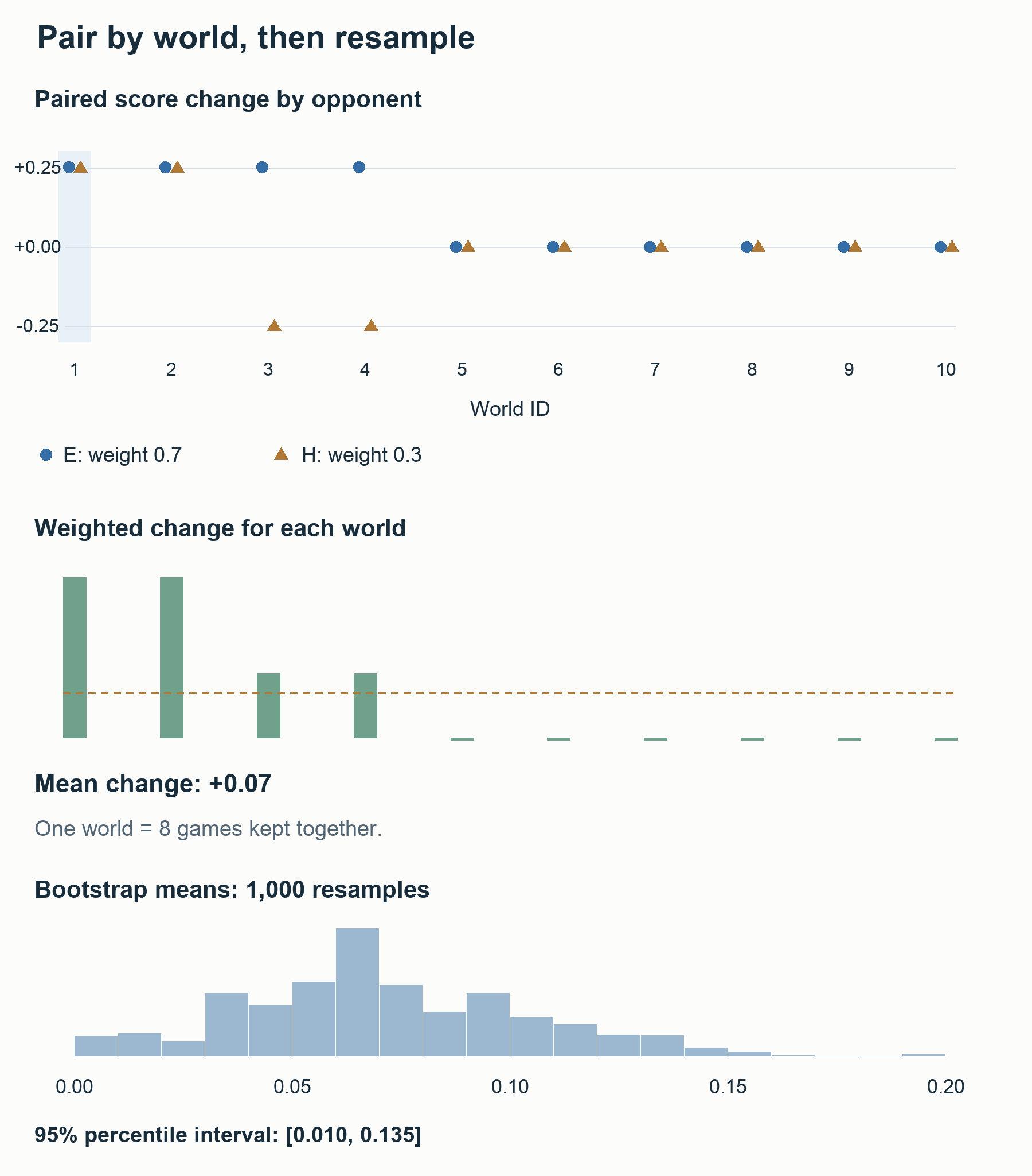
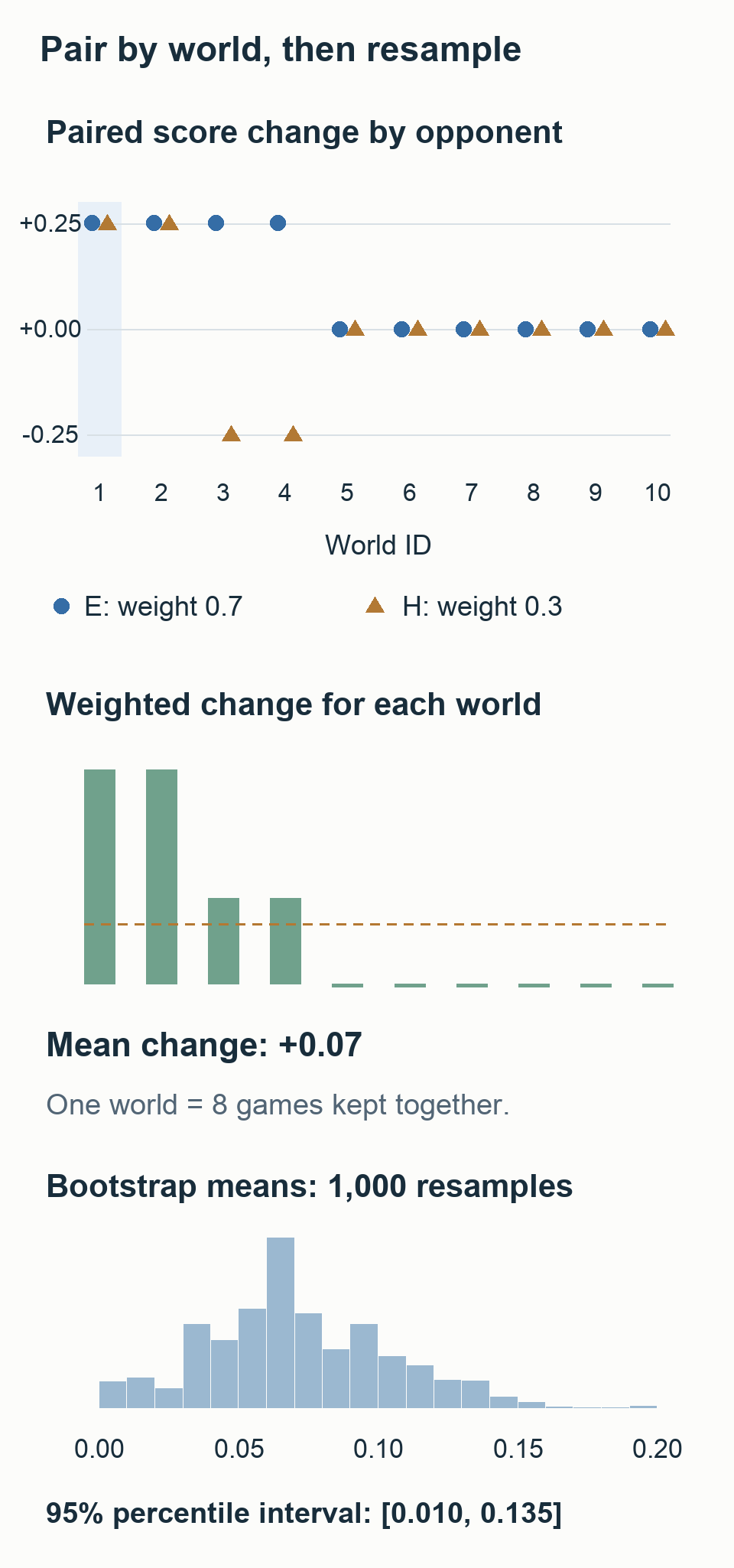
Even a +0.07 average could depend on having sampled favorable worlds. The statistical bootstrap resamples existing worlds with replacement. This is different from the value bootstrapping in Part 2, where a next-state value prediction contributes to a current training target. Draw ten worlds at a time; some can appear twice while others are omitted. Recalculate the mean repeatedly to see how sensitive it is to the sampled worlds. No new games are generated.

Worlds 1–10 in the table are indexed 0–9 in the code. For example, Figure 8’s world 1 against E is pair_delta("E", 0). The following code resamples ten worlds and calculates their mean 1,000 times. Both seats, both policies, and both opponents from the same world stay together. Opponents and weights are fixed while the world sample changes, so this does not quantify uncertainty about a new opponent entering the field.

from random import Random

worlds = list(range(10))
weights = {"E": 0.7, "H": 0.3}
baseline = {}
for opponent in weights:
    for world in worlds:
        for seat in (0, 1):
            baseline[opponent, world, seat] = 0.5
candidate = baseline.copy()

for world in range(4):
    candidate["E", world, 0] = 1.0
for world in range(2):
    candidate["H", world, 0] = 1.0
for world in range(2, 4):
    candidate["H", world, 0] = 0.0

def pair_delta(opponent, world):
    changes = []
    for seat in (0, 1):
        key = (opponent, world, seat)
        changes.append(candidate[key] - baseline[key])
    return sum(changes) / 2

group_means = {
    opponent: sum(pair_delta(opponent, w) for w in worlds)
    / len(worlds)
    for opponent in weights
}
world_changes = [
    sum(weights[o] * pair_delta(o, w) for o in weights)
    for w in worlds
]
estimate = sum(world_changes) / len(worlds)

rng = Random(2026)
bootstrap = []
for _ in range(1000):
    sampled = rng.choices(world_changes, k=len(worlds))
    bootstrap.append(sum(sampled) / len(sampled))
bootstrap.sort()

def percentile(sorted_values, q):
    position = (len(sorted_values) - 1) * q
    left = int(position)
    right = min(left + 1, len(sorted_values) - 1)
    fraction = position - left
    return (sorted_values[left] * (1 - fraction)
            + sorted_values[right] * fraction)

lo = percentile(bootstrap, 0.025)
hi = percentile(bootstrap, 0.975)
assert len(baseline) == len(candidate) == 40
assert set(candidate.values()) <= {0.0, 0.5, 1.0}
print("games / world clusters:", 80, len(worlds))
print("E / H:", *(round(group_means[o], 3) for o in weights))
print("weighted change:", round(estimate, 3))
print("bootstrap interval:", round(lo, 3), round(hi, 3))

The output includes weighted change: 0.07 and bootstrap interval: 0.01 0.135. pair_delta() averages the seat differences; world_changes combines E and H within a world using weights 0.7 and 0.3. Because the weights are fixed, resampling this world-level summary is equivalent to resampling the original result clusters together.

The values being resampled are [0.25, 0.25, 0.10, 0.10, 0, …, 0]. This preserves the pairing rather than drawing 80 individual games independently. The code sorts 1,000 means, then percentile() interpolates the values at their 2.5th and 97.5th percentiles. It assesses how the mean can vary with the worlds included in the sample. It does not mean a candidate improves in one new world with probability 95%.

The bootstrap interval from this ten-world toy example is not a universal acceptance rule. In practice, consider the world count, how well the tested opponents represent the field, and how often candidates have been selected. The example establishes how 80 outcomes become ten clusters and how weights enter the final mean.

Do not inflate the independent sample count

The 719 turns in one game are not 719 independent observations of win or loss. A pair of seat assignments also shares a world. Keep related outcomes together when calculating uncertainty.

When every opponent is tested in the same worlds, resample a world’s policy, opponent, and seat results as a whole. This is cluster bootstrap: related observations are sampled together. If each opponent uses independently sampled worlds, resample world clusters within each opponent. This quantifies sampling uncertainty for the specified opponents. The risk of different opponents appearing must be examined by adding other families or versions, or by changing the assumed opponent composition.

Checking only whether an interval’s lower endpoint exceeds zero can miss practical value. Set a minimum useful effect beforehand when releasing a tiny improvement carries substantial cost. Conversely, a wide interval containing zero may mean the current sample cannot distinguish improvement. It does not immediately establish equality or inferiority. Consider effect size, uncertainty, regressions in important opponent groups, and remaining cost together.

Selecting the best development result out of 100 candidates creates optimism through selection itself. All 100 do not need a huge final evaluation. Use inexpensive internal scores and a development panel to narrow the set, then confirm one frozen candidate under fresh conditions.

Bank differences diagnose mechanisms; match scores decide outcomes

My bank can increase by 5,000 while the opponent earns an extra 7,000, leaving me worse off. Earning another 20,000 in a landslide win while losing several close games can improve mean bank balance and reduce match score.

Record both players’ banks, revenue by product, investment timing, production, and unsold stock alongside match score. Bank differences help diagnose which economic process changed. If the objective is match outcomes, that diagnostic alone is not a promotion criterion.

The author of the low-compute BC gold-medal retrospective reports that a larger model beat a particular baseline 92–36 in a fresh evaluation yet was weaker live. Beating one opponent convincingly and being strong across styles are different conclusions.

6. Use BT ratings and leagues without losing the matchup table

Bradley–Terry models win probability from the difference in two policies’ strengths. In the basic form without a separate draw model, equal estimated strengths imply 50% win probability, and the stronger policy’s probability rises as the gap grows. The S-shaped function converting that difference to a probability between 0 and 1 is a sigmoid. BT can summarize many direct matches in an ordering and help allocate evaluation to uncertain matchups.

One number cannot fully describe cyclic relationships such as rock–paper–scissors. Rankings are also unstable when two policy groups have no connecting matches or there are too few opponents. Draw handling, priors, and uncertainty assumptions affect the result. Keep BT as a supplementary summary and preserve the underlying policy-by-opponent scores.

A league collects policies, matches them repeatedly, and tracks opponent-specific results. The Pokémon TCG population RL writeup describes a league of policies and decks that allocated more evaluation to less certain matchups. Its opponent frequencies should not be transferred to Kaggriculture; the useful lesson is how evaluation was organized.

Training need not use only the latest copy of the current model as its opponent. A small pool can include the current model, older checkpoints, strong public programs, and other styles. This helps identify cases where training only to beat the latest model causes losses to return against old opponents, or produces strength against only one style.

PFSP, or prioritized fictitious self-play, is a family of methods that adjusts training-opponent frequencies using opponent-specific results. More experience can be allocated to difficult opponents or those offering useful learning progress. AlphaStar used a league with different roles, including agents that sought weaknesses. DeepMind’s league explanation

A first project does not need the complete AlphaStar league. Start with a small fixed pool and per-opponent records, then add selection rules if the policy starts losing to opponents it previously beat. Choosing H for 50% of training because it is difficult does not justify giving H 50% of the deployment evaluation weight.

Use exploitability, vulnerability to a best-response strategy, carefully too. An attack policy may demonstrate a weakness without establishing which of all possible opponents can exploit it most severely. With a limited pool, report a discovered weakness or the worst result against tested attack policies instead.

7. Measure one complete update cycle before renting GPUs

Is there a suitable computation for the GPU?

In BC, batched neural-network inference, loss calculation, and backpropagation fit GPUs well. PPO benefits from batched inference across environments and neural-network updates. If the environment is implemented with array operations in a system such as JAX, state transitions for many games can also run on the GPU.

CPU performance may matter more when comparing strategy tables with only a few adjustable parameters in a C++ simulator, or fitting a small ridge regression. If the GPU is idle, identify the expensive computation before making the model larger.

The single-5090 tenth-place solution connected a JAX environment and policy. The winning public implementation connects a Rust environment, JAX policy, and C++ teacher. Both used GPUs, but their CPU/GPU boundaries differ. Choose the structure after measuring the bottleneck in the actual competition. The winning implementation’s runtime and components

Does the fast environment match the official one?

If a fast simulator handles trade quantities, resource ordering, or terminal rewards differently, a policy can exploit that discrepancy. Before training, compare state transitions from the same initial states and actions. Include cash shortages, insufficient inventory, simultaneous purchases, and the final turns, rather than only ordinary games.

Do not compare only the final hash. Make it possible to identify the first step and field that diverge. When the official engine changes, align versions and rerun the relevant tests. Record rules that have not yet been checked. Start with the actions being learned and important edge cases, rather than waiting for a mathematical proof of every possible behavior.

Then measure these components separately.

Component	Units and checks
Raw-data preprocessing	Games/second, cache size, RAM, repeated work
Environment stepping	Steps/second including observation and mask construction
Policy inference	Neural inference time at the actual rollout batch size
Transfer and synchronization	CPU/GPU copying and waiting
Learning update	Backpropagation and optimizer time at the actual minibatch size
Saving and evaluation	Checkpoints, log I/O, and development matches

An environment running at 100,000 steps/second does not imply the full training pipeline runs at that rate. Measure a complete cycle with the actual network, decoder, observation construction, and storage. Separate initial compilation and setup from repeated execution speed.

Define the unit of a step as well. A Kaggriculture game advances the world 719 times and contains 1,438 decisions across both seats. The same run can appear twice as fast depending on which count is used. Record VRAM use, batch size, and engine version with throughput so comparisons are meaningful.

GPU work is often asynchronous: the CPU can return after scheduling work. End a timing measurement only after the GPU computation has actually completed. Otherwise the measurement can capture scheduling rather than inference. Synchronization inserted to time individual components can remove overlap present in the original pipeline, so measure the complete cycle separately too.

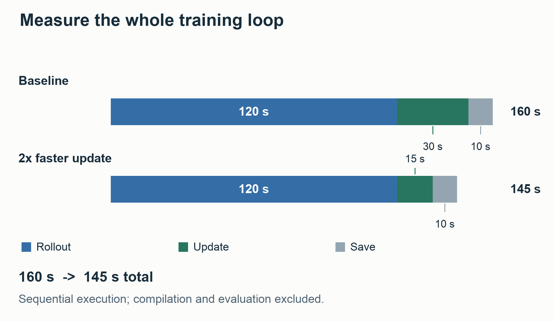
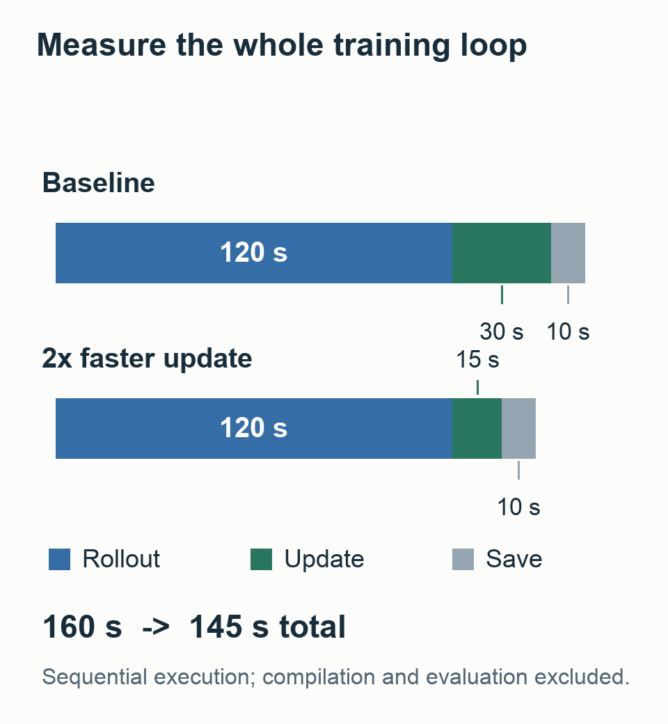
Suppose rollout, update, and saving run sequentially and take 120, 30, and 10 seconds. One cycle takes 160 seconds. Doubling only the GPU update speed reduces the total to 145 seconds. Overlapping work changes the timing calculation, but also requires tracking how stale the experience-collection policy is relative to the current training policy. Start with small batches collected and updated in sequence to establish correctness.

Figure 9. Under sequential execution, doubling update speed reduces the total from 160 to 145 seconds. Blue is rollout, green is update, and gray is saving. Bar lengths are proportional to time. Initial compilation and separate evaluation are excluded.

Work through a hypothetical rental budget

Assume a fictional rate of KRW 1,000 per hour and a 600-second development evaluation every ten updates. At 160 seconds per cycle, 100 updates require 16,000 seconds, with another 6,000 seconds for evaluation. That is about 6.1 hours, or approximately KRW 6,100 of compute. Data preparation, initial compilation, recovery margin, separate CPU resources, and storage cost extra.

Even if training cycles complete twice as fast, keeping the separate 6,000 seconds of evaluation makes the total 14,000 seconds, about 3.9 hours. Savings depend on which work became faster. These prices and times are budgeting assumptions, not hardware quotations.

Before booking a long run, ask what decision this expenditure will make possible. Do not reserve hundreds of PPO updates when a small BC policy cannot even finish a game. Once a cycle works correctly and improvement appears, use its measured time to budget a larger run.

8. Complete the first experiment, one stage at a time

There is no need to automate stages A–G in the first run. Establish A with an existing program, follow one teacher record into a training example in B, then move to C. Save each stage’s output and attach the next computation only after its checks pass. When something fails later, resume from the last working stage.

A — Fix the objective and strongest simple baseline

Inputs: competition rules, scoring, runtime limits, and available strong programs. Record whether match score or revenue is the objective, how opponents are sampled, and which of multiple submissions is evaluated. Decide whether the model chooses one complete plan or worker and market commands every turn.

Computation: small reproducible matches and runtime measurements. Output: a baseline with fixed code, engine, and decoder versions. Do not compare only against a weak earlier policy because it is convenient; include the strongest simple policy already available. Run the same package again under the same conditions and confirm correct operation before moving on.

B — Build a small teacher dataset and action pipeline

Inputs: complete game records and metadata from teacher programs with verified versions. Computation: select teacher seats, split by game, and inspect observation, action, execution, and label conversions. Output: a small manifest, defined input/output formats, and training samples that can be explained by hand.

Check that labels preserve actions such as hiring, placement, and selling that affect later operation. For one recorded decision, convert a valid action to a label and decode it back into a command. Fix the conversion if quantity, order position, or resource use changes. Invalid command strings need not be reconstructed verbatim, but deleting their slots must not shift later orders. The full archive does not need to be converted to training arrays at the start.

C — Play a small BC policy directly

Inputs: checked teacher data and a small model. Computation: run BC, first checking that it can fit a small training set, then examining loss and important actions on games outside training. Output: a policy that plays to completion from current observations rather than reading a tape. If even training examples cannot be matched, inspect data conversion and loss first. If training is fitted but development examples fail, investigate which conditions and teachers are missing.

Play the model directly and follow hiring, production, transport, and sales. If it predicts recorded teacher actions accurately but actual play collapses, do not immediately increase model size. Check whether the decoder changes commands incorrectly, incompatible teacher strategies were mixed, or the model’s own mistakes led to unfamiliar states. A sufficiently strong BC policy can be evaluated as a candidate without PPO.

D — Choose a generation method for the actual failure

Inputs: losses of BC or the existing policy, and alternative strategies used by strong players. Computation: separate the causes of defeat and identify which method can change the relevant behavior. Output: one hypothesis for the next experiment.

Observed limitation	First computation to try
A good strategy exists but is not learned correctly	Revise labels, features, BC, or teacher mixture
No recovery experience after the policy’s own mistakes	Collect visited states and relabel with a teacher where possible
Every available strategy is weak	Generate a new complete teacher, plan, or action representation
A few meaningful quantities such as investment intensity can be adjusted	Search, CEM, or ES that samples near promising combinations
A strong starting policy exists and its responses could improve	PPO on fresh rollouts
The plan is good but commands conflict	Fix scheduling, resource reservations, and execution code

To label a new state visited by my policy, a teacher program or search procedure must be able to accept that state and calculate a good action. Someone else’s old replay cannot supply targets for states it never contains.

After discovering weaknesses in tomato-heavy and skewed-shop worlds, the winning team improved its teacher planner, generated complete demonstrations in those worlds, and returned to BC. It did not try to solve every weakness by assigning more PPO compute. Targeted teacher-data generation

E — If PPO is appropriate, trace one update

If BC or plan search alone produced the candidate, skip this stage and proceed to independent evaluation in F. PPO is not a mandatory sequel to BC.

Inputs: a fixed collection-policy version, an opponent pool, and new worlds. Computation: save action log probabilities, value predictions, masks, and rewards, then perform one advantage-based update. A reward scores an action’s outcome for the learning objective. Output: a checkpoint traceable to the experience used to update it.

Immediately after collection, recompute log probabilities with the same masks and compare them with stored values. If post-processing forcibly changes an action, do not train it under the original action’s probability. If value predictions are inaccurate, fit the critic first while preserving the actor. Do not mix records from other old policies as though they were fresh PPO data from the current policy.

In the first update, establish that the computation is connected correctly. Stored old probabilities and advantages remain fixed while gradients are calculated through the current policy to its weights. A loss without NaNs and a changed weight file are insufficient evidence of success. Nor should every update be required to increase win rate. After a predefined short training stage, inspect important behavior and development matches. If probability calculations are wrong or operation suddenly collapses, return to the last sound checkpoint and diagnose the cause.

Round-trip the probabilities before updating

Suppose actions are BUY, WAIT, and SELL, with BUY unavailable because cash is insufficient. Network logits [2, 1, 0] become probabilities [0, approximately 0.731, approximately 0.269] when normalized only over legal actions.

In the code below, chosen represents one sample in which WAIT was selected. It is not a rule to always choose WAIT in a real rollout. Fix one action so only its collection-time and recomputed probabilities are compared.

Before any weight change, the same state, action, and mask should yield the same probability. The PPO ratio must therefore be 1. Saving logits but reconstructing a different mask changes that ratio even though the weights have not changed.

import math

actions = ["BUY", "WAIT", "SELL"]
logits = [2.0, 1.0, 0.0]
mask = [False, True, True]
chosen = actions.index("WAIT")

def masked_probs(values, allowed):
    assert len(values) == len(allowed)
    legal_values = [v for v, ok in zip(values, allowed) if ok]
    if not legal_values:
        raise ValueError("no legal action")
    offset = max(legal_values)
    terms = [
        math.exp(v - offset) if ok else 0.0
        for v, ok in zip(values, allowed)
    ]
    total = sum(terms)
    return [term / total for term in terms]

collect_probs = masked_probs(logits, mask)
old_logprob = math.log(collect_probs[chosen])
repeat_probs = masked_probs(logits, mask)
new_logprob = math.log(repeat_probs[chosen])
ratio = math.exp(new_logprob - old_logprob)
assert math.isclose(ratio, 1.0, abs_tol=1e-12)

wrong_probs = masked_probs(logits, [True, True, True])
wrong_ratio = wrong_probs[chosen] / collect_probs[chosen]
print("chosen probability:", round(collect_probs[chosen], 6))
print("unchanged-policy ratio:", round(ratio, 6))
print("wrong-mask ratio:", round(wrong_ratio, 6))

The chosen action probability is 0.731059, the unchanged-policy ratio is 1.0, and the wrong-mask ratio is 0.334759. Before measuring the effect of a policy change, verify that the same policy is being evaluated under the same probabilities. The tolerance 1e-12 is for this small Python floating-point calculation. For float32 or mixed precision, choose a tolerance appropriate to the numerical format.

A policy that chooses workers and market orders sequentially changes masks according to resources left by earlier choices. Recompute conditional log probabilities in that same order, then sum them. Identical final commands do not establish identical probability calculations. Observations, policy version, masks, and inference settings must all agree.

If post-processing changes WAIT to SELL, WAIT’s probability cannot be stored as SELL’s old log probability. Define how altered actions enter training, or apply the same constraints during collection and training so actions are selected consistently in the first place.

F — Confirm one candidate under fresh conditions

Inputs: one candidate chosen from development results, with predefined opponent weights. Computation: paired matches against the baseline in both seats, using worlds excluded from training and selection, with checks for opponent-specific regressions. Output: effect size, uncertainty, and a reason to accept, defer, or reject.

Test the final candidate with the same sampling or argmax, post-processing, masks, and numerical precision as the actual submission. Improvement when sampling according to probabilities does not guarantee improvement under argmax, which always takes the most likely action. A small reversal in the top two probabilities can change the same opening decision in every game.

Suppose the first market decision has only investment and waiting as choices.

Policy	Investment probability	Wait probability	First submitted action under argmax
Before update	0.49	0.51	Wait
After update	0.51	0.49	Invest

Sampling increases the investment frequency by two percentage points. Under argmax, the first action at this observation flips every time. This happens even though KL(before ∥ after) is only about 0.0008 nat. Changed cash, labor, and production can then make the whole game different. Small KL and small changes in deployed behavior are not equivalent.

There is no universal sufficient game count. Choose it according to the improvement to be distinguished, variation across worlds, opponent count, and runtime cost. If the expected effect is too small to separate within the budget, return to a hypothesis capable of a larger change or defer judgment.

G — Package deployment and recovery together

Inputs: the accepted candidate and final CPU package. Computation: complete games in the official environment, first-call and normal-call timings, memory, initialization, and failure fallback checks. Output: the final package and hash, reproduction commands, and the evidence behind its selection.

Resuming training needs more than weights. Save optimizer state, learning-rate schedule, RNG state, opponent pool, manifest, completed and incomplete rollouts, and code and engine versions. Record whether the last experience batch has finished its updates. Ending a rental should not leave ambiguity about what to resume, duplicate an update on the same experience by accident, or lose intermediate work.

The winning team’s public evaluator runs both seat assignments for each seed, but does not exactly reproduce Kaggle’s container scheduling and time accounting. Local correctness and correct behavior in the actual submission environment require separate checks. The public evaluator’s scope

9. Write a one-page experiment specification

Suppose the hypothesis is a strong BC policy underinvests in tomato-demand worlds. A record like this gives reasons to start, continue, and stop computation.

Question
  Does adding complete teacher demonstrations for tomato-demand
  worlds reduce that weakness while preserving normal-world strength?

Baseline and changes
  Baseline: frozen BC checkpoint and deployment decoder
  Change: same model and budget, BC with targeted teacher data added
  Control: BC with the same amount of general teacher data added

Inputs
  Teacher code/seats, engine, data hashes, game-level split
  Definition of tomato-demand worlds and normal-world samples

Computation
  Small label check → small training run → development matches
  Paired confirmation in fresh worlds for one promising candidate

Decision
  Match-score change and interval in target worlds
  Regressions beyond acceptable limits in normal worlds/opponent groups
  Whether tomato investment, harvest, and revenue actually changed

Budget and stop conditions
  Measured training/evaluation cost and total limit
  Stop immediately on label mismatch or execution collapse
  Do not scale up without a promising change within development budget

Recovery
  Baseline checkpoint, optimizer, RNG, and restart commands

Compare adding targeted teacher data with adding the same quantity of general data. This separates the effect of more data from the effect of learning the missing operating strategy. More candidates also mean more confirmation cost, so do not combine every possible modification at the start.

Match the total training budget while recording update counts and how often each example is reused. Equal epochs do not imply equal computation when dataset size increases.

10. Know where to return when results are poor

Symptom	Inspect first	Do not immediately increase
Cannot fit even a small sample	Time alignment, labels, loss masks, outputs and decoder	Full dataset or model size
Matches teacher states but collapses in its own games	First consequential divergence, resource conflicts, missing data for visited states	PPO duration
Operates normally but remains far below strong players	Whether teachers or the menu contain a good strategy at all	Complexity of a selector over weak options
Worsens immediately after PPO	Old log probability, masks and automatic action repair, critic, reward scale	Parallel environment count
Improves in development but fails fresh confirmation	Selection bias, opponent families, new worlds, decoder	Repeated runs on the same development panel
Bank increases but match score falls	Opponent bank, close games, product-specific market effects	Bank-reward weight
Training is fast but complete cycles are slow	CPU environment, observations, transfers, I/O, evaluation	GPU count

It is easy to attach a plausible story to one loss. Check whether the problem recurs across games, whether a change actually removes it, and whether it creates losses elsewhere. That evidence can justify changing the next training run.

When inspecting logs, align both players’ cash, inventory, actions, model action probabilities and value predictions, actual trade quantities, and cancellation reasons on one timeline. A drop in predicted value is a clue, not proof that the move at that instant caused the problem. Trace preceding investments, movement, and inventory changes.

Give every metric a purpose in the first week’s notes

The number of metrics can be overwhelming at first. Return is the sum of rewards from a given point onward. Do not judge from mean return alone; inspect strategy generation, learning, execution, and actual match results separately.

Metric	Conditions to record	First question when it worsens
Mean return	Reward definition, collection policy, opponent versions and weights	Did opponents get easier, or did the policy change?
Critic error	Return targets in the same reward units and evaluation samples	Are reward units, termination, and next-value handling correct?
Entropy	Action head and number of legal choices	Did choice collapse, or did the legal set shrink?
KL from the previous policy	Identical observations and masks, comparison direction	Which states or actions changed most?
Executed-behavior metrics	Timing and success of hiring, expansion, harvests, and sales	Are intended actions canceled or automatically altered?
Fresh confirmation score	Fixed opponents, new worlds, submission decoder	Did better training metrics translate into better matches?

Assess critic accuracy by comparing prediction $V(s_t)$ with the return target $G_t$ at the same observation. For example, take the mean absolute difference:

\[\operatorname{MAE}_V =\frac{1}{N}\sum_{t=1}^{N}|V(s_t)-G_t|.\]

Here, $N$ is the number of observations evaluated.

Fitting training targets and predicting outcomes on new games are different achievements. Record whether targets are Monte Carlo returns summing actual rewards to termination, or GAE targets that incorporate value estimates. Changing reward units also changes error magnitudes, so do not compare numbers from different experiments without accounting for their scales.

Entropy describes how probability is distributed over actions. It is higher when three actions have similar probabilities and lower when one dominates. Zero entropy is not a problem if insufficient cash leaves only one legal action. Averaging together important purchase decisions and states with no real choice can hide why entropy fell.

Suppose the following changes appear in a fictional training notebook. Collection means come from the opponent pool at each point; fixed-evaluation returns use the same separate opponent composition. Intermediate rewards are 0, terminal rewards are +1 for a win, 0 for a draw, and −1 for a loss, with discount $\gamma=1$. Return in this table is the mean terminal reward per game.

The purchase head is the model component that outputs purchase actions. Assume at least four available choices here, allowing higher entropy than Part 2’s three-action example. The missed required hire rate is measured only in states selected in advance from teacher actions and execution conditions. It is neither the no-hire rate over all states nor disagreement with an optimal action selected in hindsight.

Record	Collection mean return	Fixed-evaluation return	Evaluation critic MAE	Purchase-head entropy	Missed required hires
Start	+0.10	+0.10	0.80	1.20	2%
Fifth update	+0.28	+0.02	0.50	0.30	22%

Under these win/draw/loss rewards, mean return equals 2 × mean match score − 1. The fixed-evaluation change +0.10 → +0.02 corresponds to match score 0.55 → 0.51. These are the same results on different scales. They do not mean the competition’s BT rating fell by 0.08.

Collection return and critic error alone suggest improvement. Yet performance against the fixed evaluation opponents worsened, and important hires were missed more often. First inspect masks and action probabilities in states where hiring was possible, and why the decoder canceled commands. A fall in entropy is not by itself a reason to raise its bonus coefficient or run PPO longer.

If a mask incorrectly blocked hiring, fix the condition. If hiring was legal but its probability disappeared after learning, inspect that state’s advantage, reward, and teacher KL. If no demonstration showed a better opening investment in the first place, different data or a strategy-generation method is needed. Identical metrics can require different code changes depending on the cause.

End a training note with one check and the change that will follow from its result, rather than train more. For example: Compare masks with actual command handling in states where hiring is possible. If they disagree, fix that before training; otherwise inspect the advantage at those states. This keeps the next run from repeating the same computation without a concrete purpose.

11. Study by building one working artifact at a time

There is no need to learn every RL algorithm first. Being able to explain and implement these six pieces is enough to start a small competition loop.

1. One game’s state transitions. Follow observations, actions, rewards, and termination by hand for a few decisions. Read the engine and construct a small reproducible example.
2. Classification and BC. Learn logits, softmax, cross-entropy, minibatches, and gradients. Train on a small teacher dataset and play the resulting policy to completion.
3. Value and advantage. Calculate return and its difference from the expected result along one game’s record. Explain why a game’s reward does not by itself evaluate each individual action.
4. PPO probability calculations. Trace one update and locate old/new log probabilities, ratio, clipping, entropy, KL, and value loss.
5. Opponents and evaluation. Build a small matrix covering self-play, past checkpoints, opponent weights, paired comparisons, and separation of development from final confirmation.
6. Broader generation methods. Then apply ES/CEM, plan search, teacher distillation, or leagues to a specific weakness.

The important outcome is what can be checked directly, not pages read. It should be possible to follow a path through the code and data: this observation led to this action, and this result changed the weights this way. Once a small cycle works, a GPU can execute it more often and under more varied conditions.

On the first day of the next competition, I would fill in these three fields before writing more code.

Where behavior better than the current policy will be generated:
What new information is needed to learn or evaluate that behavior:
The one decision this computation will enable us to accept or reject:

Specific answers make it easier to choose among BC, PPO, strategy tables, and plan search. If the process only keeps reranking existing candidates, revisit the first field. If it creates many new candidates but their strength is uncertain, return to the second and third.

---

Part 1 — From Benchmarks to Strategy Generation · Part 2 — How BC, PPO, and Plan Search Improve Play