Kaggriculture RL, Part 1: From Benchmarks to Better Strategies

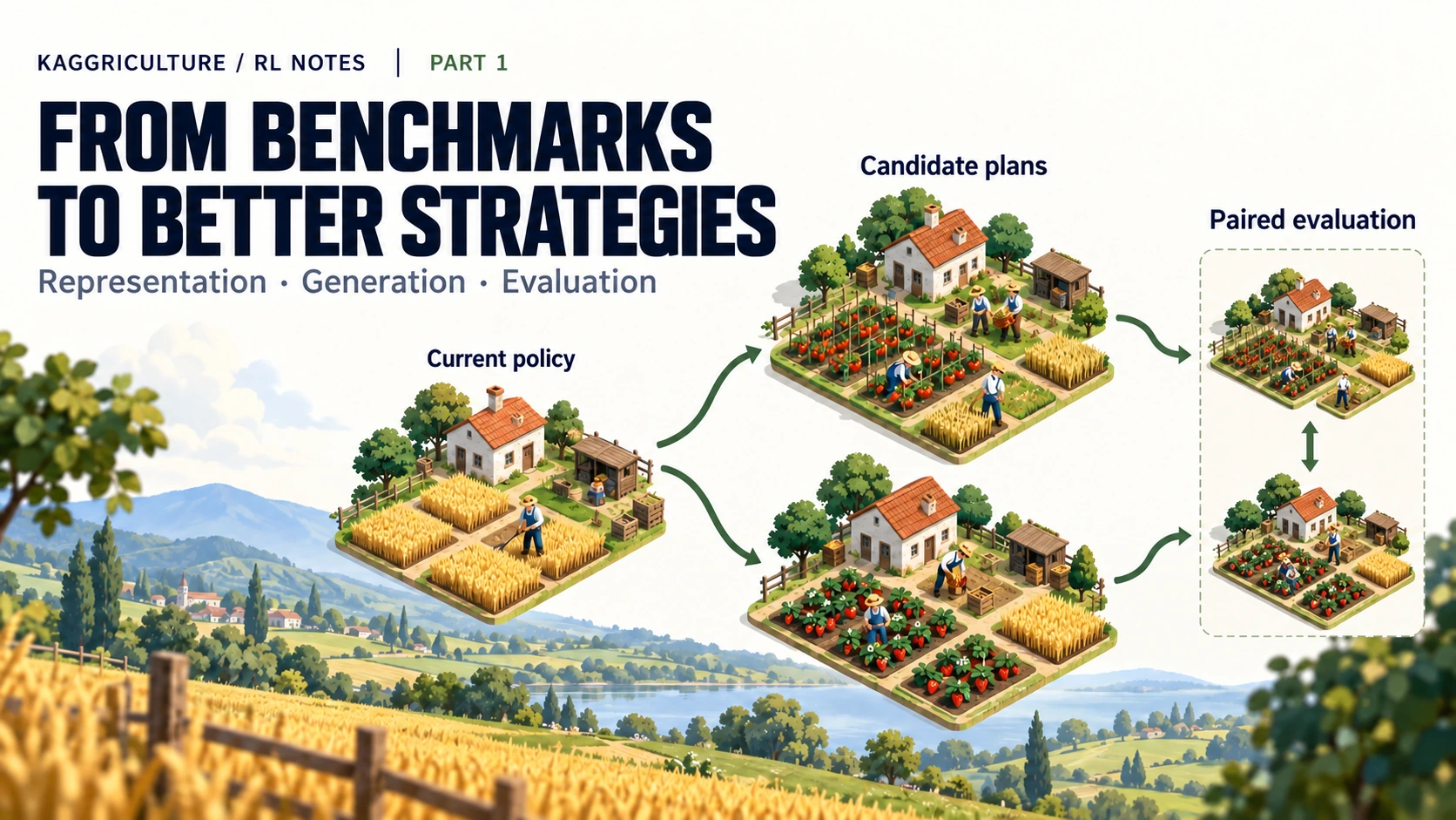
The most frustrating part of Kaggriculture often came after a benchmark finished. I could identify the opponents we lost to, the point at which we ran short of cash, and the crops that generated too little income. I kept looking for ways to change the strategy. What remained unclear was what to change, and how to make the computer find a better version. More games were available, but I did not know which changes those games should help me discover.

In my first working note, I designed a farm economy by hand and analyzed the action records of public games. Reading competitors’ writeups and code after the competition made the differences in strategy generation much clearer. Some work involved editing individual actions. Other teams learned from strong demonstrations, changed action probabilities using new games, or searched for plans that changed labor, land, and crops together.

I had trained models too. I had attempted to generate whole plans and found useful rules in live losses. What was missing was a reliable connection between those activities. Were any of the available alternatives actually better? Could the agent execute a promising plan all the way through? Would a local improvement survive against the latest opponents? Those were separate questions, and each needed its own evidence.

1. Turning an early hire into revenue

Kaggriculture compares the final bank balances of two farms after 30 days. Each day has 24 turns, during which the agents handle production, movement, transport, and market orders. Both players trade in the same market, so one player’s sales affect the prices available to the other. More cash now does not necessarily mean a stronger position. One farm may have invested in land and crops; the other may be accumulating inventory it will not manage to sell in time.

Consider hiring an extra worker early in the game. The hiring cost is paid immediately, and the worker stays for that day only. If the worker is needed tomorrow, the agent must hire again. Without useful work to assign, the extra hire is simply an expense. Buying land is similar: seed purchases, watering, harvesting, and transport must follow before the investment produces revenue.

To recover the money spent on hiring and land, the agent must complete the later tasks on time. Lower market prices—or neglecting existing livestock to work the new plots—can make the whole plan unprofitable.

“Plant more tomatoes” therefore requires decisions about which worker goes where and does what. A neural network does not remove that requirement. Either the training data must contain such an operation, or the search procedure must be able to construct the tasks that make it work.

Bank balance, margin, and match outcomes

A final balance of 100,000 loses to 100,001. A balance of 70,000 beats 60,000. Since shop and market conditions vary across games, the farm that earned 100,000 is not necessarily stronger than the one that earned 70,000. I will use final bank margin = our final balance − the opponent’s final balance, shortened to margin.

At least three measurements need to remain separate.

Measurement	Question it answers	Main use
Our final balance	How much money did we make under these conditions?	Production, investment, and logistics analysis
Final bank margin	How much more did we make than this opponent in this game?	Economic gaps and close-game analysis
Win, draw, or loss	How often do we finish ahead?	Competitive strength and final evaluation

The average margin can increase without changing the match score if the agent merely earns more in games it already wins comfortably. Conversely, a small amount of extra money can be valuable if it turns several narrow losses into wins. There is no fixed conversion from “extra coins” to rating points. We need to know which opponents and conditions produced a different outcome.

2. Policies, learners, and benchmarks

A policy is a program that chooses the next action from the information available to the agent. “Buy a cow if there is enough money” is a policy. So is a table that selects a recorded sequence of actions—a tape—from the shop configuration. A neural network is another kind of policy. The word does not imply a particular neural architecture.

A learner changes the policy’s parameters using data or new experience. A benchmark runs the policy under specified conditions and measures its performance. A person can improve a policy by reading benchmark results and editing rules, but then the person must invent the next change each time.

Reinforcement learning (RL) uses the reward received after actions to learn better choices. Behavior cloning (BC) instead uses a strong player’s actions as supervised targets. PPO is an RL algorithm that updates a policy using rewards from its own experience. BC and PPO can be used in sequence, but they learn from different signals.

Breaking the program into components makes it easier to identify what needs to change.

Component	Kaggriculture example	What goes wrong when it is inadequate
Strategy representation	Daily goals, complete routes, action probabilities, selection tables	Strategies outside that representation cannot be produced.
Candidate generation	Rearranging routes, changing crops, sampling policy actions	The system keeps proposing similar weak alternatives.
Execution	Turning goals into movement, work, and market orders	A plan with attractive predicted revenue collapses during execution.
Evaluation and learning	Future-profit estimates, BC loss, PPO updates	The system improves something other than the actual objective.
Independent evaluation	New conditions and opponents that react to our actions	Improvement in development games is mistaken for competitive strength.

A GPU can accelerate the expensive parts. It cannot supply a missing candidate generator, make an unexecutable plan work, or correct the objective being optimized. An evaluation panel is a collection of opponents and conditions. A reactive opponent reads the changed situation and responds—for example, when our actions alter the market. It must be treated differently from an opponent that only replays recorded commands.

Observations are not the engine’s full state

A person looks at the game screen; a program receives an observation through the game’s API. In Kaggriculture, that includes information such as the current day and hour, our cash, crops, worker positions, and public market prices and shops. The engine may also hold future random draws or private opponent information. The agent does not necessarily receive all of it.

Someone reading a replay can see the end of the game. That does not make “choose tomatoes on day one because a tomato shop will appear later” a usable submission policy. Complete records can supply training targets and outcome analysis, but the policy’s inputs must be restricted to information available when the decision was made.

We can write a policy as $a_t\sim\pi_\theta(\cdot\mid o_t,m_t)$. Read it as: “Use the information and memory available at time $t$ to calculate action probabilities, then draw an action.”

Symbol	Meaning	Farm example
$t$	Decision time	Turn 0, 1, or 2
$o_t$	Observation received at that time	API inputs such as day, cash, worker positions, and prices
$m_t$	Memory saved from earlier turns	Previous prices or earlier decisions
$a_t$	Selected action	Hiring, movement, harvesting, or market orders
$\pi_\theta$	Policy determined by parameters $\theta$	Behavior defined by rule coefficients, a selection table, or neural weights

The information after $\mid$ is what the decision is conditioned on. The dot $\cdot$ is the place occupied by possible actions. The symbol $\sim$ means drawing an action from the calculated distribution. A rule that always chooses the same action can also be viewed as a policy assigning probability 1 to that action. Basic RL definitions

Adjusting parameters to data is called fitting. A loss is a quantity defined so that training tries to reduce it. In BC, assigning a low probability to the teacher’s action produces a larger loss. A gradient describes how the loss changes when each parameter changes slightly. An optimizer uses that gradient to update the parameters. The practical question is still: Which parameters change in this experiment, and which actions can those parameters change?

A small farm, one decision at a time

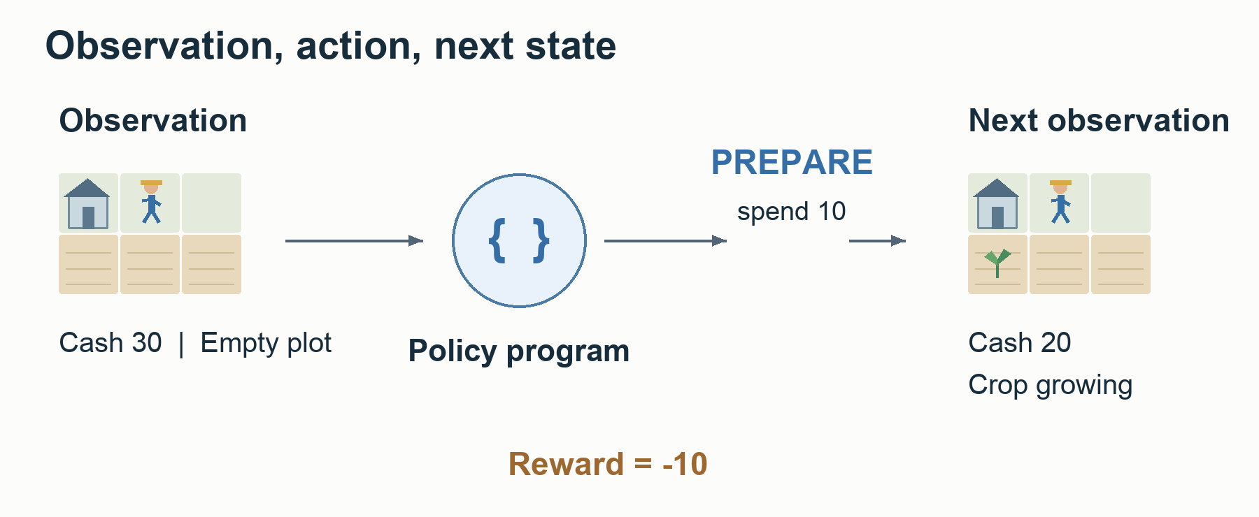
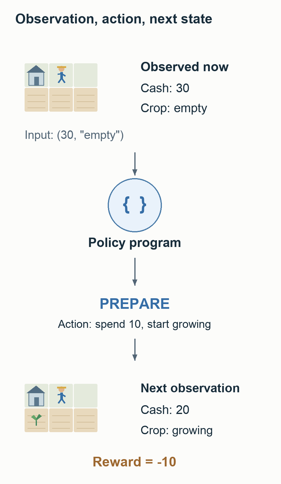
Reduce the farm to three decisions. Start with 30 cash, spend 10 on preparation, tend the crop, then sell the harvest for 20. This is a hypothetical small game without dates, market prices, or hiring costs. Its complete state is visible in the observation.

Decision time	Current state	Action	Next state	Reward
0	Cash 30, empty plot	Prepare	Cash 20, growing crop	−10
1	Cash 20, growing crop	Tend	Cash 20, ripe crop	0
2	Cash 20, ripe crop	Sell	Cash 40, finished	+20

The environment takes an action and produces the next state. This is a transition. A reward is numerical feedback assigned to that result for learning. Here it equals the cash change, but we could instead give +1 only at the end of a win. The game rules and the reward attached to their results are different design choices.

Term	Meaning in this small farm
Turn or step	One action followed by an advance of the environment, such as preparing the plot
Episode	One complete game, from the empty plot to termination: 3 transitions and 4 states here
Trajectory	A time-ordered record of state → action → reward → next state
Rollout	Running a policy to collect trajectories, or the resulting experience; it can cover multiple games
Batch	Samples processed together in one computation; the three transitions could form one batch
Epoch	One pass through a defined dataset; two passes over these three samples are 2 epochs
Update	One parameter change by the optimizer using the calculated gradient

An epoch is not an update. With 1,000 data rows and batches of 100, one epoch usually involves 10 updates. Gradient accumulation, which combines gradients from several batches before applying an update, changes that relationship. A rollout is not necessarily a complete game either: collection can stop partway through an episode. Count games, transitions, sample reuse, and parameter updates separately.

Figure 1. The first transition in the small farm. The policy chooses PREPARE from the current observation; the environment spends 10 and changes the crop state. The reward is the cash change, −10.

From a game to one record

This code runs the game and records its transitions. policy chooses an action from the current state, while rules determines how cash and the crop phase change. We use cash_change directly as reward. The policy has already been specified: this is experience collection, not yet an algorithm that learns better actions.

rules = {
    "empty": ("prepare", -10, "growing"),
    "growing": ("water", 0, "ripe"),
    "ripe": ("sell", 20, "done"),
}
policy = {"empty": "prepare", "growing": "water", "ripe": "sell"}
state = (30, "empty")
trajectory = []
for turn in range(3):
    cash, phase = state
    action = policy[phase]
    expected, cash_change, next_phase = rules[phase]
    assert action == expected
    next_state = (cash + cash_change, next_phase)
    reward = cash_change
    done = next_phase == "done"
    trajectory.append((state, action, reward, next_state, done))
    state = next_state
print("actions:", [row[1] for row in trajectory])
print("final cash:", state[0])

The output is actions: ['prepare', 'water', 'sell'] and final cash: 40. The first record, ((30, 'empty'), 'prepare', -10, (20, 'growing'), False), says: start with 30 cash and an empty plot, prepare, receive reward −10, and move to a growing crop with 20 cash. The final False means the game has not ended yet.

Records can have the same shape but serve different learning purposes depending on who played.

Source	Information used for learning	Question
A strong player’s teacher trajectory	Observation–action pairs such as (cash 30, empty plot) → prepare	Can the model predict the teacher’s action from this information?
A rollout from our current policy	Our action, its probability and value prediction at collection time, and subsequent rewards	Was the result better than expected, and how should the action probability change?

This distinguishes BC samples made from a teacher’s records from PPO experience generated by our own policy. To extend the code into a PPO collector, we would also store logprob, the logarithm of the selected action’s probability, and value, the predicted outcome from that state. Later updates need the probabilities and expectations that applied when the experience was collected.

Evaluating a cost now and revenue later

A return sums rewards from the current point onward. The rewards in this game are −10, 0, +20, which sum to +10. Write the reward at time $t$ as $R_t$ and the return from that point as $G_t$. With discount factor $\gamma=0.9$, a reward one step away receives weight 0.9, and one two steps away receives weight $0.9^2$. At the start:

\[\begin{aligned} G_0&=R_0+\gamma R_1+\gamma^2R_2\\ &=-10+0.9\times0+0.9^2\times20\\ &=6.2. \end{aligned}\]

Cash did not increase by 6.2. It increased from 30 to 40; the discounted return is 6.2. With $\gamma=1$, the return would be +10 too. Looking only at the initial expense of −10 would miss the revenue that follows. RL has to estimate how current choices contribute to later results.

A critic predicts the return obtained by continuing with the policy from the current state. That prediction is called the value. At the start of this farm, its target is neither the current cash of 30 nor the final cash of 40, but the return of 6.2 under the chosen discount. In a real game the future is uncertain, so the model learns this expectation from multiple experiences.

Kaggriculture does not rank agents by the cash-reward sum in this small example. The final balance determines each game’s outcome, and results against multiple opponents contribute to the final evaluation. Keep the training reward, the return predicted by the critic, and the competition objective distinct. That distinction also matters when comparing the single-5090 solution’s money-difference reward with the winning team’s win/loss reward.

3. Candidate quality and the limits of selection

Suppose three programs already exist: the original plan, livestock expansion, and crop expansion. Assume the following expected match scores in four situations, with a win worth 1, a draw 0.5, and a loss 0.

Observed situation	Original plan	Livestock expansion	Crop expansion
Spare cash and labor	0.50	0.80	0.30
Low cash, plenty of empty land	0.50	0.20	0.80
Feed secured, crop market oversupplied	0.50	0.70	0.30
Feed scarce, crop market in demand	0.50	0.10	0.70

If all four situations occur equally often, always using the original plan gives 0.50, always expanding livestock gives 0.45, and always expanding crops gives 0.525. Choosing the best program in every situation would give $(0.8+0.8+0.7+0.7)/4=0.75$. This idealized reference, which knows all the values, is an oracle. These alternatives offer something to gain from context-dependent selection.

Copying the table’s rows and columns into Python makes the calculation easy to inspect.

scores = [
    [0.50, 0.80, 0.30],
    [0.50, 0.20, 0.80],
    [0.50, 0.70, 0.30],
    [0.50, 0.10, 0.70],
]
fixed = [sum(row[col] for row in scores) / len(scores)
         for col in range(3)]
oracle = sum(max(row) for row in scores) / len(scores)
print("fixed:", [round(value, 3) for value in fixed])
print("oracle:", round(oracle, 3))

The output is fixed: [0.5, 0.45, 0.525] and oracle: 0.75. The expression sum(row[col] ...) keeps one program fixed across situations; max(row) selects the best program within each situation. The gap between the strongest fixed strategy and the oracle is $0.75-0.525=0.225$. In practice, however, we do not know the expected scores exactly, and the observation may not distinguish every relevant situation. There is no guarantee that a learned selector can recover the entire gap.

If both alternatives are weaker than the original plan in every situation, a better selector will merely choose the original plan more often. Before enlarging the selection network, ask whether the available choices contain a better alternative at all.

An experiment can run each alternative against the same opponents and initial conditions, then compare:

1. The best score obtained by keeping one policy fixed across the whole sample.
2. The score obtained by selecting the best alternative in each cell after observing the results.

The second is a hindsight oracle. Our hypothetical table assumed known expected scores, but a single real game supplies only an outcome of 0, 0.5, or 1. Selecting the maximum after seeing those outcomes also selects lucky results. An actual policy cannot see future results, so the hindsight oracle is not an achievable-performance guarantee.

It is still diagnostic. If no better alternative appears even in the same sample, generating better plans is more urgent than learning to select among them. If a gap does appear, we must separately test whether the relevant situation is identifiable before the decision and whether the advantage persists in new games.

The output determines what can change

Two models can both read cash and farm information while controlling very different parts of the strategy.

Program	Input	Output	Who operates the farm afterward?
Simple selector	Observation at the selection point	One plan name: original, livestock, or crops	An already implemented controller
Per-turn action policy	Current observation and memory	Hiring, movement, work, and market commands	The policy reads the next observation and decides again
Planner	Current farm, resources, and time constraints	A coordinated plan for workers, tasks, routes, and trades	An executor converts the plan into commands

Write out input → adjustable parameters → output → execution. If the network outputs only the ID livestock expansion, existing code still decides where the cow goes and who feeds it. Changing the selector’s weights cannot create a barn that its chosen controller never builds. A per-turn policy can change more decisions, but needs data covering a full season and an execution design that prevents conflicting resource use. A planner constructs those coordinated tasks as an explicit plan.

4. What our models actually learned

One of my learners was an option-value model: it selected a work plan for the current situation. We ran the original policy and an alternative to the end from the same decision point, then used their match-score difference and margin change as targets. Ridge regression predicted the gain from features, numerical inputs extracted from the observation such as cash and staffing. This learned which alternative to choose; it did not update per-turn action probabilities with PPO.

The basic regression calculation is features multiplied by coefficients to predict a gain. Set aside the margin auxiliary target for a moment and predict only the match-score difference from the existing policy. Suppose the features are scaled to 0–1, with spare cash $x_1=0.8$ and labor burden $x_2=0.2$, and the fitted coefficients are:

\[\begin{aligned} \widehat y&=0.05+0.10x_1-0.20x_2\\ &=0.05+0.08-0.04\\ &=0.09. \end{aligned}\]

The prediction $\widehat y=0.09$ means an expected match-score improvement of 9 percentage points over the existing policy, not 9 competition rating points. If it exceeds the acceptance threshold, the agent executes the alternative; otherwise it keeps the original policy. Fitting finds coefficients that bring predictions closer to the gains $y$ observed in games. Ridge regression adds a penalty to discourage excessively large coefficients. These numbers illustrate the calculation; the actual model used more features.

Reading the ridge equation used in the implementation

$X$ stacks the features of multiple decision situations as rows, and $y$ contains the gains observed from the alternative in actual matches. $W$ is a matrix of sample weights specifying how much importance to give each sample. The fitted coefficients are collected in $\widehat\beta$, while $\lambda$ sets the penalty strength. The superscript $\mathsf T$ denotes transposition, which exchanges rows and columns; $^{-1}$ denotes a matrix inverse.

\[\begin{aligned} \widehat\beta&=(X^\mathsf{T}WX+\lambda R)^{-1}X^\mathsf{T}Wy,\\ R&=\operatorname{diag}(0,1,\ldots,1). \end{aligned}\]

The actual implementation had two target columns: match-score difference and a margin auxiliary target. The same equation fitted coefficients for each. The auxiliary target divided the margin change by 10,000 and applied tanh to bound it between −1 and 1. At selection time, the predicted match-score difference was combined with the weighted auxiliary prediction. The main example simplifies this to a prediction of match-score difference alone.

The first entry of penalty matrix $R$ is 0 because the intercept was not penalized. The code solved the linear system using np.linalg.solve rather than explicitly constructing an inverse. It fitted many coefficients together instead of manually changing one coefficient and running matches after each edit.

We also collected new games with the changed policy and fitted again. But fitting the existing table well does not guarantee good selection in new games. Overfitting occurs when a model follows incidental patterns in its training data and performs poorly on new data. Training fit and competitive performance under new conditions need separate evaluation.

This model learns, “Which plan is better here?” Its control range differs from a network choosing movement, hiring, planting, and selling every turn. Neither is universally superior. The useful alternative must lie within the model’s output space.

The selector predicts how much better an alternative is than the existing plan. A PPO critic predicts the return from continuing with the current policy. Their reference points and reward units differ, so an output of 0.1 does not mean the same thing in both models.

4.1 Training gains versus performance in new games

The fertilizer-selection experiment on September 13 performed two fits. The recorded mean match-score differences from the existing policy were:

Evaluation	Match-score difference
First model: evaluation on the option table used for fitting	+0.14583
First model: evaluation on newly collected experience	−0.06250
Second model: evaluation on the option table used for fitting	+0.09375
Second model: execution under new development conditions	−0.03125

The dataset contained 192 rows, but only 64 distinct decision situations and 16 seed groups. A seed initializes random-number generation. Testing multiple alternatives and seats under conditions derived from the same seed adds rows without adding independent world conditions. Two differently named alternatives also produced the same observed actions, and the anticipated fertilization of carrots never occurred.

It would therefore be wrong to diagnose this as “we never performed an RL update.” We did change the model. But it learned the gains of small alternatives from limited experience, and performance deteriorated under new conditions. We first needed to check whether the alternatives behaved differently and how much distinct experience we had collected.

4.2 The alternative itself lost value

The September 14 cashflow experiment combined funding, hiring, fertilization, harvesting, transport, and sales into a carrot-production plan. Of the first 160 conditions compared, the plan activated in 95. In every one of those 95, the margin was lower than with the existing policy. Across the experiment, 528 valid games were run; no model was fitted.

The newly assigned work yielded 154 additional carrots. But assigning labor there displaced 531 carrots and 396 wheat from the original routes. The extra hiring expense also exceeded the fertilizer savings. Counting only the new work’s harvest misses the production sacrificed to do it: the opportunity cost of labor.

In this case, the plan needed revision before the model needed more parameters or epochs. Total production had to increase, or the new work had to earn more than the work it displaced. Accurately rejecting unprofitable alternatives is useful, but it does not by itself produce a new high-scoring strategy.

4.3 A selector beat the weak baseline and lost to the strong one

On September 15, we trained a model to select between two controllers. On the same newly evaluated confirmation sample after training, the mean match scores were:

Policy	Mean match score
Always use C2	0.291667
Learned selector B	0.541667
Always use V43	0.666667

Looking only at the +0.25 improvement over C2 makes this appear successful. Always using V43 was better, however: the learned selector scored 0.125 lower on this sample. Its fallback to the weaker C2 when inputs fell outside the training range contributed to the loss.

A baseline is the reference used to judge a new model’s value. Comparing only with a weak predecessor can exaggerate an improvement. A strong fixed policy, a simple selection rule, and the program already in use should all be considered before the added complexity of a selector is justified.

These measurements were checked against the retained execution records and result documents. The experiment IDs are rl_system_20260913, cashflow_rl_20260914, and strategy_learning_20260915. These match-score differences do not tell us how much the official final rating would have changed.

5. Execution constraints and action decoding

We also built a whole-plan generator and a new executor. An early implementation mistakenly counted wheat in one worker’s bag as shared inventory available to everyone. The accounting said enough feed existed, but the worker responsible for feeding could not obtain it. Other failures included buying animals without placing them and failing to continue the existing policy’s later investments.

Earning a plan’s predicted revenue requires actual tasks to satisfy concrete conditions.

Intended operation	What execution requires
Feed a cow tomorrow	The responsible worker must collect feed from its actual location and arrive in time.
Plant on newly purchased land	The worker must arrive after the land and seeds become usable.
Increase production with an extra hire	The assigned route must fit movement, work, and return travel into the day.
Sell the harvest	Bags and storage must hold it, and DROP timing, market-order processing, and the sale deadline must be respected.
Maintain existing production	The plan must account for watering, feeding, and care displaced by the new work.

Execution is part of the policy. A decoder turns model outputs into actual commands. If it emits commands with different meanings from those used during training, or a trade that worked in the simulator fails in the official engine, the learned strategy is not being executed as trained.

A useful first test is an action → label → action round trip. Convert the teacher’s action into its training label, reconstruct a command, and execute it under the official rules. Check that cash, inventory, and crop changes follow the recorded behavior. If this fails, repair the conversion and execution before asking how accurately the network predicts the labels.

6. Tapes, behavior cloning, and plan search

The same strong replay can be the starting point for different methods. What they preserve and how they act in a new game differ.

Method	What is stored or learned	What happens in a new game
Tape	An ordered sequence of actions from a particular game	Replay the command at that time, with some corrections.
BC	A model predicting teacher actions from observations	Choose the next action from the information available now.
Plan search	A representation of crops, tasks, and routes, plus an evaluator	Construct and compare executable plans from the current state.

Tapes were not useless. Our agent inherited a design that selected complete routes from public replays according to observed conditions. We also tested a separate complete tape. The question was whether its commands would remain executable with different cash, markets, and opponents. A tape that passed an evaluation panel later went 11 wins to 37 losses against another actual router.

Instead of replaying “hire at step 144,” BC predicts a hiring probability from the current day, cash, staffing, and farm information. Even after choosing a different action from the teacher, it reads the observation produced by that choice. Making the next decision from feedback on one’s own actions is called closed-loop control. It does not guarantee recovery in unfamiliar states. Small errors can accumulate, so prediction accuracy on teacher records and performance when the learned agent plays a full season need separate tests.

A planner generates candidates from the current state and estimates their results. A planner that changes only the worker count searches a different strategy space from one that jointly changes hiring, land, planting, and routes. Even a good evaluator cannot improve the investment strategy if the necessary candidates are never generated.

7. What did people automate?

People still made many decisions. They designed inputs, action representations, teacher selection, training opponents, and rewards. They inspected losses to identify problems such as too little tomato production or storage failures.

But they did not necessarily edit every parameter by hand and run a large benchmark after every change. Different methods automated different kinds of changes.

BC learns a strong player’s complete operation

Collect records of a strong agent hiring, buying land, planting, tending, and selling. The network changes many weights together so that each observation assigns a higher probability to the teacher’s action. A person need not write hundreds of thousands of rules saying, “Move left in this state.”

The BC loss does not, by itself, ask the model to outperform its teacher. Actual play must establish how much of the operation it learned, whether it executes rare hiring and land orders, and whether it can recover after an imitation error.

PPO adjusts probabilities using the policy’s own outcomes

Run new games with the current policy, then use better- or worse-than-expected results to adjust action probabilities. Again, the updated weights are shared across many states. The critic estimates the return from a state; the advantage estimates how much better or worse the experience was than that expectation. These estimates guide action evaluation rather than treating every action in a winning game as a good choice. PPO paper

A large benchmark is not required after every update. Rollouts and updates repeat while training health is monitored; saved intermediate weights, or checkpoints, undergo development evaluation. The chosen final candidate is then tested on conditions reserved separately. Frequent training changes and final candidate validation need different schedules and budgets.

ES and CEM search small sets of strategy parameters

If only a few numbers control the strategy—early investment, target livestock counts, or how many days ahead to consider when selling—we can sample and evaluate combinations. Evolution Strategies (ES) aggregate the results of random perturbations to move in a promising direction. The Cross-Entropy Method (CEM) shifts the sampling distribution toward regions containing successful candidates. Neither requires an exhaustive sweep of every value one coordinate at a time. Original ES paper

Candidate games still cost time. If increasing the livestock target does not cause the executor to adjust feed and labor, search can keep proposing infeasible combinations. We must first check that changing the parameters produces a coherent change in the actual operation.

Structured search avoids repeating the whole season

Decomposing crop growth and daily work into smaller problems, or recalculating only changed routes, reduces the cost of evaluating a candidate. The winning planner approximates future production, labor costs, and sales this way while proposing different worker counts and crop configurations. Its score is an internal prediction. The completed program still needs actual games under the official rules against reactive opponents. Winning planner implementation

8. How high-scoring teams improved their strategies

The team that finished 10th with a single RTX 5090 trained BC from strong replays, ran the environment on the GPU to gather new experience, and applied PPO. Its public code connects the environment, observations, legal actions, learning, and CPU submission. It is an example of completing the learning-to-execution loop on one GPU. Time and resource figures are author-reported; reading the code does not independently reproduce the ranking.

The 24th-place team spent its early weeks on rules, planning, and sales optimization before learning strong agents’ operations through BC. Training the selling-horizon table over millions of games used CPUs; the final submission was BC-based. Consumer GPUs supported repeated training, but Colab A100 was also used to pretrain the trunk, the shared representation component of the final model. “A small GPU learned one table and won gold” would misrepresent that sequence.

That team also compared adding tomato rules with changing teacher data. A rule that changed a planting action provided limited improvement. Adding demonstrations from a newer teacher that already operated tomatoes successfully taught the associated labor allocation and production as well. This did not mean discarding all corrections: some supporting rules remained in the final submission.

The 116th-place team used CPU simulations to build a table that selected among hundreds of complete tapes based on observed shops. It improved the application of existing good plans rather than inventing a new farming operation from scratch. Acquiring strong plans and choosing well among them are distinct contributions.

A high rank achieved with a method does not identify how many points each component contributed. Teacher data, representational capacity, execution, opponent composition, and training volume all differed. To apply these lessons in another competition, ask which failure the team found and what it changed next, rather than stopping at an algorithm’s name.

9. What our benchmarks missed

A September 15 audit found that 1,024 of 2,048 games had been spent against Land and Plateau opponents the two policies already beat almost every time. Each policy won 254/256 in that portion. More seeds against familiar weak opponents provide little information about how to challenge the latest strong agents.

Comparing later live records showed that local results agreed with live results for the same exact program versions present in the panel. Most losses came from newer programs outside it. The issue was not that all local games were wrong: our predictions for tested opponents held up, but we had not tested enough of the actual competition.

Our claim that logs had been used only for monitoring was also inaccurate. Live losses generated guard, fertilizer, and carrot rules. The narrower problem was filtering strong opponents by whether they differed from our code in only a few actions. This made small corrections easy to absorb, but excluded agents using different investment and production systems from the start.

Finding better plans required a different question:

Under which conditions does a currently strong submission version pull ahead, and through which investments and task assignments? Can we learn that operation as a policy or plan using the observation available now?

This does not mean mixing every strong player’s logs. We need to establish the version, information available at the time, correct action labels, and compatibility of the operations being learned. Reactive matches are still necessary at the end. But similarity to our current code should not be mistaken for strategic value.

10. Failure diagnosis and experiment selection

Before starting another training run, identify where the process is blocked.

Symptom	Inspect first	Purpose of the next computation
Every alternative is weaker than the existing policy.	Total production changes and displaced work	Generate a better plan.
A useful alternative exists, but the selector misses it.	Observations, distinct decision situations, and fallback	Learn when to choose it.
Predicted profit is high, but execution collapses.	Cash, inventory locations, routes, and deadlines	Make the intended operation executable.
BC accuracy is high, but autonomous play is weak.	Rare decisions, action–label conversion, and states after our errors	Improve features, decoder, or teacher data.
PPO loss changes, but actions and performance do not.	Actual probability changes, critic, reward, and exploration	Diagnose the learning signal.
The policy is strong only on the old panel.	Current opponent versions and their reactivity	Change what is evaluated.

Without this diagnosis, we repeat the same treatment for different problems: enlarge a model when its choices are poor, add training when execution is wrong, or add seeds to an old panel after the opponents have changed.

Two diagnostic exercises

Exercise 1. Compare an existing policy and two alternatives in the same 32 world–opponent conditions. In every condition, both alternatives receive a lower match score than the existing policy. Should the first step be adding more training rows and enlarging the selection network?

Answer

The current sample contains no better alternative to select. Investigate total production changes and work displaced by the proposed plan, then generate a plan that can outperform the existing policy. This does not reject every possible strategy. It distinguishes poor available choices from poor selection among those choices.

Exercise 2. A BC model matches 99% of actions in teacher records. In a new game it misses an early hire, then assigns work to a nonexistent worker and production collapses. Is training longer on the same teacher data sufficient?

Answer

Average accuracy can conceal rare but important hiring errors. After missing the hire, the model also enters a different state from the teacher's records. First inspect the hiring label and decoder, and how the inputs and commands handle missing workers. Collect the first divergence and the subsequent states, then decide whether to add teacher data, teach recovery, or learn from new rollouts. Matching teacher records and completing games well with one's own policy are separate evaluation tasks.

A useful starting point is one small experiment carried through to completion: select executable actions from observations, record experience, change the policy through learning, and test whether it is better under new conditions. Connecting that loop makes failure informative about the next computation.

In the next competition, I want to ask “What candidate that I do not have now will exist after this computation?” before asking how many games a GPU can run. Then I need to specify how the candidate will execute and which games, unused for training or selection, will establish whether it is stronger.

Further reading and sources

• Part 2 — How BC, PPO, and search produce better strategies: actual code, learning signals, and future-value calculations for coordinated worker, land, and crop changes.
• Part 3 — From logs to learning and credible evaluation: joining data, separating evaluations, measuring GPU work, and an execution sequence for the next competition.
• The first Kaggriculture working note: farm economics, early policies, and replay analysis.
• Single-5090 implementation, winning implementation, 24th-place writeup, and 116th-place writeup.
• Basic RL concepts, original PPO paper, and original ES paper.

Our experiment measurements were checked against docs/rl_system_20260913.md, docs/cashflow_rl_20260914.md, docs/strategy_learning_20260915.md, docs/field_audit_20260915.md, and their result files retained in the project. Live scores at project closure are distinct from official final results after the competition. A closure snapshot was not used to infer the official final rank.